Sparse linear models

Using LASSO to interpret the results

Setup

# Colab setup
import os

if os.getenv("COLAB_RELEASE_TAG"):
    import subprocess
    subprocess.run('wget https://raw.githubusercontent.com/luigibonati/mlcolvar/main/colab_setup.sh', shell=True)
    cmd = subprocess.run('bash colab_setup.sh EXAMPLE', shell=True, stdout=subprocess.PIPE)
    print(cmd.stdout.decode('utf-8'))

# IMPORT PACKAGES
import torch
import lightning
import numpy as np
import matplotlib.pyplot as plt
import mlcolvar.utils.plot

# Set seed for reproducibility
torch.manual_seed(1)

<torch._C.Generator at 0x7f74b7608950>

In this notebook we show how sparse linear models can be used to interpret NN-based ones, in the spirit of this paper. As example we train an autoencoder CV on the intermolecular aldol reaction from the examples, and we try to interpret the results, using both a classification or a regression linear model.

Train a ML CV

As an example we train a simple autoencoder on the given datasets.

from mlcolvar.io import create_dataset_from_files
from mlcolvar.data import DictModule

filenames = [ "https://raw.githubusercontent.com/luigibonati/data-driven-CVs/master/aldol/1_unbiased/INPUTS.R",
              "https://raw.githubusercontent.com/luigibonati/data-driven-CVs/master/aldol/1_unbiased/INPUTS.P" ]

n_states = len(filenames)

# load dataset
dataset, df = create_dataset_from_files(filenames,
                                        filter_args={'regex':'cc|oo|co|ch|oh' }, # select contacts
                                        create_labels=True,
                                        return_dataframe=True,
                                        )

datamodule = DictModule(dataset,lengths=[0.8,0.2])

Class 0 dataframe shape:  (5001, 43)
Class 1 dataframe shape:  (5001, 43)

 - Loaded dataframe (10002, 43): ['time', 'cc2.0', 'cc2.1', 'cc2.2', 'oo2.0', 'co2.0', 'co2.1', 'co2.2', 'co2.3', 'co2.4', 'co2.5', 'ch2.0', 'ch2.1', 'ch2.2', 'ch2.3', 'ch2.4', 'ch2.5', 'ch2.6', 'ch2.7', 'ch2.8', 'ch2.9', 'ch2.10', 'ch2.11', 'ch2.12', 'ch2.13', 'ch2.14', 'ch2.15', 'ch2.16', 'ch2.17', 'oh2.0', 'oh2.1', 'oh2.2', 'oh2.3', 'oh2.4', 'oh2.5', 'oh2.6', 'oh2.7', 'oh2.8', 'oh2.9', 'oh2.10', 'oh2.11', 'walker', 'labels']
 - Descriptors (10002, 40): ['cc2.0', 'cc2.1', 'cc2.2', 'oo2.0', 'co2.0', 'co2.1', 'co2.2', 'co2.3', 'co2.4', 'co2.5', 'ch2.0', 'ch2.1', 'ch2.2', 'ch2.3', 'ch2.4', 'ch2.5', 'ch2.6', 'ch2.7', 'ch2.8', 'ch2.9', 'ch2.10', 'ch2.11', 'ch2.12', 'ch2.13', 'ch2.14', 'ch2.15', 'ch2.16', 'ch2.17', 'oh2.0', 'oh2.1', 'oh2.2', 'oh2.3', 'oh2.4', 'oh2.5', 'oh2.6', 'oh2.7', 'oh2.8', 'oh2.9', 'oh2.10', 'oh2.11']

from lightning.pytorch.callbacks.early_stopping import EarlyStopping
from mlcolvar.utils.trainer import MetricsCallback
from mlcolvar.cvs import AutoEncoderCV

# define model
n_input           = dataset['data'].shape[-1]
nodes             = [40,30,30,1]
nn_args           = {'activation': 'shifted_softplus'}
options           = {'encoder': nn_args}

model = AutoEncoderCV(nodes, options=options)

# define trainer
trainer = lightning.Trainer(accelerator='cpu', max_epochs=500, logger=None, enable_checkpointing=False)

# fit
trainer.fit( model, datamodule )

GPU available: True (cuda), used: False
TPU available: False, using: 0 TPU cores
IPU available: False, using: 0 IPUs
HPU available: False, using: 0 HPUs
/home/lbonati@iit.local/software/mambaforge/envs/mlcolvar110/lib/python3.10/site-packages/lightning/pytorch/trainer/setup.py:187: GPU available but not used. You can set it by doing `Trainer(accelerator='gpu')`.
/home/lbonati@iit.local/software/mambaforge/envs/mlcolvar110/lib/python3.10/site-packages/lightning/pytorch/trainer/connectors/logger_connector/logger_connector.py:67: Starting from v1.9.0, `tensorboardX` has been removed as a dependency of the `lightning.pytorch` package, due to potential conflicts with other packages in the ML ecosystem. For this reason, `logger=True` will use `CSVLogger` as the default logger, unless the `tensorboard` or `tensorboardX` packages are found. Please `pip install lightning[extra]` or one of them to enable TensorBoard support by default

  | Name    | Type          | Params | In sizes | Out sizes
-----------------------------------------------------------------
0 | loss_fn | MSELoss       | 0      | ?        | ?
1 | norm_in | Normalization | 0      | [1, 40]  | [1, 40]
2 | encoder | FeedForward   | 2.2 K  | [1, 40]  | [1, 1]
3 | decoder | FeedForward   | 2.2 K  | ?        | ?
-----------------------------------------------------------------
4.4 K     Trainable params
0         Non-trainable params
4.4 K     Total params
0.018     Total estimated model params size (MB)

/home/lbonati@iit.local/software/mambaforge/envs/mlcolvar110/lib/python3.10/site-packages/lightning/pytorch/loops/fit_loop.py:293: The number of training batches (1) is smaller than the logging interval Trainer(log_every_n_steps=50). Set a lower value for log_every_n_steps if you want to see logs for the training epoch.

Epoch 499: 100%|██████████| 1/1 [00:00<00:00, 28.51it/s, v_num=52]

`Trainer.fit` stopped: `max_epochs=500` reached.

Epoch 499: 100%|██████████| 1/1 [00:00<00:00, 19.80it/s, v_num=52]

LASSO

Sparsity in linear models can be enforced via L1 regularization on the weights. In this way, we can obtain a parametrization of the model with only a few non-zero coefficients, which is more interpretable. The number of non-zero coefficients depends on the magnitutde of the regularization strength.

LASSO classifier

We can interpret the metastable states that we found in the CV space by training a lasso classifier on the labeled dataset, and finding a minimal set of descriptors that can distinguish one state from another.

Under the hood, this is achieved using the LogisticRegressionCV from scikit-learn (sklearn.linear_model); note that CV here refers to cross-validation, since different models are trained in a range of regularization values.

Scoring function

To find the optimal value of the regularization strength, we use the following scoring function, which balances the accuracy and the number of non-zero coefficients. In particular, it retains a feature only if it increases the classification accuracy by more than 1%. In addition, a minimum number of features can be requested.

\[\text{score} = - (1-\text{accuracy})*100 - \left|n-\text{min\_features}\right|\]

Assign labels

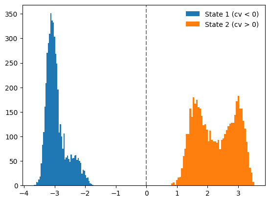
Being a classification task, we need a labeled dataset. As an example, here we use the CV trained above to assign the labels. Indeed, if we visualize the CV distribution, we realize that there are two distinct states, which we can label based on the value of the CV (greater or smaller than 0).

# evaluate CV
with torch.no_grad():
    s = model(dataset['data']).cpu().numpy()

# assign labels
labels = np.zeros_like(s)
labels[np.argwhere(s<0)] = 1
labels[np.argwhere(s>0)] = 2

dataset['labels'] = torch.Tensor(labels).squeeze(-1)

#plot
plt.hist(s[labels==1],bins=50,label='State 1 (cv < 0)')
plt.hist(s[labels==2],bins=50,label='State 2 (cv > 0)')
plt.axvline(0,linestyle='dashed',color='grey')
plt.legend(frameon=False)
plt.show()

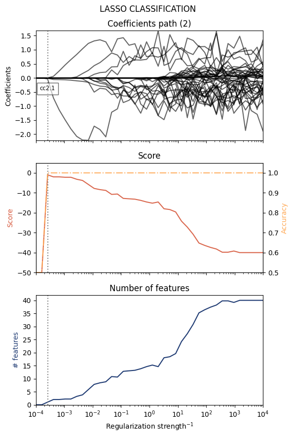
Train classifier

from mlcolvar.explain.lasso import lasso_classification

classifier, feats, coeffs = lasso_classification(dataset, plot = False)

======= LASSO results (2) ========
- Regularization : 0.00025719
- Score          : -1.00
- Accuracy       : 100.00%
- # features     : 1

Features:
(1) cc2.1        : -0.442826
==================================

Plot

In order to find the best classifier, we can look at the following plots as a function of the (inverse) regularization strength.

1. values of the coefficients

2. score

3. number of features

from mlcolvar.explain.lasso import plot_lasso_classification

plot_lasso_classification(classifier,feats,coeffs)

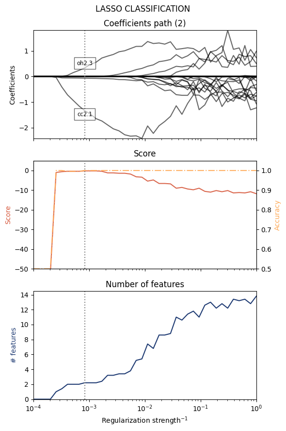
We can specify the range of the regularization parameters with the Cs argument (the inverse of the regularization strength).

from mlcolvar.explain.lasso import lasso_classification

classifier, feats, coeffs = lasso_classification(dataset, Cs=np.logspace(-4,0,40), min_features=2)

======= LASSO results (2) ========
- Regularization : 0.00083768
- Score          : -0.20
- Accuracy       : 99.80%
- # features     : 2

Features:
(1) cc2.1        : -1.545506
(2) oh2.3        : 0.454156
==================================

Or even a single value

classifier, feats, coeffs = lasso_classification(dataset, Cs = [1e-3], plot=False)

======= LASSO results (2) ========
- Regularization : 0.00100000
- Score          : -2.20
- Accuracy       : 99.80%
- # features     : 2

Features:
(1) cc2.1        : -1.668857
(2) oh2.3        : 0.531198
==================================

Alternatively, the min_features keyword can be used to request a model with a given number of features.

from mlcolvar.explain.lasso import lasso_classification

classifier, feats, coeffs = lasso_classification(dataset, min_features=3, plot=False)

======= LASSO results (2) ========
- Regularization : 0.00272833
- Score          : -0.60
- Accuracy       : 99.40%
- # features     : 3

Features:
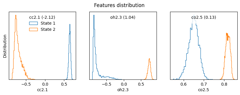
(1) cc2.1        : -2.120870
(2) oh2.3        : 1.035353
(3) co2.5        : 0.134075
==================================

Once we have found a set of relevant features, we can plot their distribution to see their values in the different states.

from mlcolvar.utils.plot import plot_features_distribution

plot_features_distribution(dataset,features=feats[2], titles=[f'{l} ({c:.2f})' for l,c in zip(feats[2],coeffs[2])])

3

LASSO regression

Another way to interpret the results is by training a linear model to approximate the non-linear CV, in terms of a few descriptors. We can do so with a lasso regressor, optimized with the following loss:

\[\frac{1}{2\ \text{n\_samples}} ||y - Xw||^2_2 + \alpha\ ||w||_1\]

Under the hood, this is achieved using the LassoCV from scikit-learn (sklearn.linear_model); note that CV here refers to cross-validation, since different models are trained in a range of regularization values.

Note that for a sparse regressor, scikit-learn uses directly the regularization strength \(\alpha\) rather than its inverse as in the sparse classifier above.

Being a regression task, we need a dataset with a “target” field, in this case this is the value of the CV.

with torch.no_grad():
    dataset['target'] = model(dataset['data']).squeeze(-1)

Train the lasso regressor

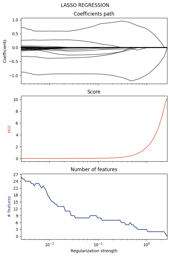
As before, we can look at the values of the cofficients, the score (in this case it is directly the objective) and the number of selected features.

from mlcolvar.explain.lasso import lasso_regression

regressor, feats, coeffs = lasso_regression(dataset, alphas=None, plot=True)

========= LASSO results ==========
- Regularization : 0.00262542
- Score          : 0.99858080
- # features     : 25

======= Relevant features =======
(1) oh2.9        : -0.860057
(2) oh2.3        : 0.785916
(3) ch2.15       : -0.308029
(4) ch2.9        : 0.243112
(5) oh2.6        : -0.124784
(6) oh2.1        : -0.111379
(7) oh2.7        : -0.082770
(8) ch2.4        : -0.079014
(9) oh2.0        : -0.072904
(10) oo2.0        : -0.066918
(11) ch2.11       : -0.059698
(12) ch2.12       : -0.059411
(13) co2.5        : 0.057554
(14) oh2.8        : -0.052454
(15) co2.2        : -0.038305
(16) co2.0        : 0.033872
(17) co2.4        : -0.018800
(18) ch2.6        : 0.017482
(19) ch2.1        : 0.008754
(20) oh2.4        : -0.007725
(21) ch2.7        : 0.007211
(22) ch2.2        : -0.005044
(23) ch2.8        : 0.001218
(24) ch2.10       : -0.000993
(25) oh2.10       : -0.000036
=================================

Here the keyword alphas (regularization strength) can be used to select a given model:

mr_regressor, mr_feats, mr_coeffs = lasso_regression(dataset, alphas=[0.5])

========= LASSO results ==========
- Regularization : 0.50000000
- Score          : 0.95937854
- # features     : 5

======= Relevant features =======
(1) oh2.9        : -1.190525
(2) oh2.3        : 0.875116
(3) co2.1        : -0.056142
(4) cc2.1        : -0.025593
(5) ch2.12       : -0.023096
=================================
Plotting is not available, as the regressor has been optimized with a single regularization value.

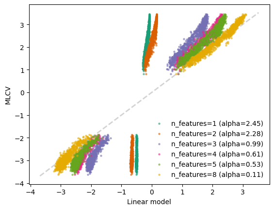
To understand the quality of the approximated CV, we can compare the linear models with different regularization strenghts with target CV. In particular, we select the alphas corresponding to different number of features

num_features = [1,2,3,4,5,8]

# we analyze the coefficient paths of the cross-validated model to find the alphas which correpond to different number of features
num_features_path_ = np.count_nonzero(regressor.coefs_paths_.T, axis = 1)

selected_alphas = []
for num_feat in num_features:
    id = np.argwhere(num_features_path_ == num_feat).min()
    alpha = regressor.alphas_[id]
    selected_alphas.append(alpha)
    print(f'num_feat={num_feat} --> alpha={alpha:.2f}')

num_feat=1 --> alpha=2.45
num_feat=2 --> alpha=2.28
num_feat=3 --> alpha=0.99
num_feat=4 --> alpha=0.61
num_feat=5 --> alpha=0.53
num_feat=8 --> alpha=0.11

# standardize inputs
with torch.no_grad():
    X = dataset['data'].numpy()
    y = dataset['target'].numpy()

from sklearn.preprocessing import StandardScaler
X = StandardScaler(with_mean=True, with_std=True).fit_transform(X)

# test different values of alpha
from cycler import cycler
fig,ax = plt.subplots()
ax.set_prop_cycle(cycler(color=plt.get_cmap('Dark2').colors))

for alpha in selected_alphas:
    regressor, feats, coeffs = lasso_regression(dataset, alphas=[alpha],print_info=False,plot=False)
    y_pred = regressor.predict(X)
    ax.scatter(y_pred[::5], y[::5],s=5,label=f'n_features={len(coeffs)} (alpha={alpha:.2f})',alpha=0.5)
    # print equation
    equation = "y="
    for f, c in zip(feats,coeffs):
        equation+=f"+{c:.3f}*{f} " if c> 0 else f"{c:.3f}*{f} "

    print(equation[:-1])

ax.set_xlabel('Linear model')
ax.set_ylabel('MLCV')
ax.plot([y.min(),y.max()],[y.min(),y.max()],linewidth=2,color='lightgrey',zorder=0,linestyle='dashed')
ax.legend(frameon=False)
plt.show()

y=-0.177*oh2.9
y=-0.322*oh2.9 +0.020*oh2.3
y=-0.985*oh2.9 +0.680*oh2.3 -0.003*cc2.1
y=-1.158*oh2.9 +0.812*oh2.3 -0.074*cc2.1 -0.015*co2.1
y=-1.183*oh2.9 +0.857*oh2.3 -0.047*co2.1 -0.044*cc2.1 -0.011*ch2.12
y=-0.953*oh2.9 +0.862*oh2.3 -0.295*ch2.15 -0.237*co2.1 +0.127*ch2.9 -0.067*ch2.12 -0.042*cc2.2 -0.001*ch2.14