TPI-DeepTDA: Chignolin mini-protein¶

Reference paper: Ray, Trizio and Parrinello, JCP (2023) [arXiv].

Prerequisite: DeepTDA tutorial.

Setup¶

[4]:

# Colab setup
import os

if os.getenv("COLAB_RELEASE_TAG"):
    import subprocess
    subprocess.run('wget https://raw.githubusercontent.com/luigibonati/mlcolvar/main/colab_setup.sh', shell=True)
    cmd = subprocess.run('bash colab_setup.sh EXAMPLE', shell=True, stdout=subprocess.PIPE)
    print(cmd.stdout.decode('utf-8'))

# IMPORT PACKAGES
import torch
import lightning
import numpy as np
import matplotlib.pyplot as plt

# Set seed for reproducibility
torch.manual_seed(42)

[4]:

<torch._C.Generator at 0x7fd09b4f46b0>

Chignolin protein¶

We first train a DeepTDA CV on the chignolin data, which is one of the examples of the TPI-Deep-TDA paper. This is a small protein often used for testing as it prvide a simple example of folding dynamics in protein. Indeed, chignolin in water presents two metastable states, folded and unfolded, and the interconversion between them involves several degrees of freedom.

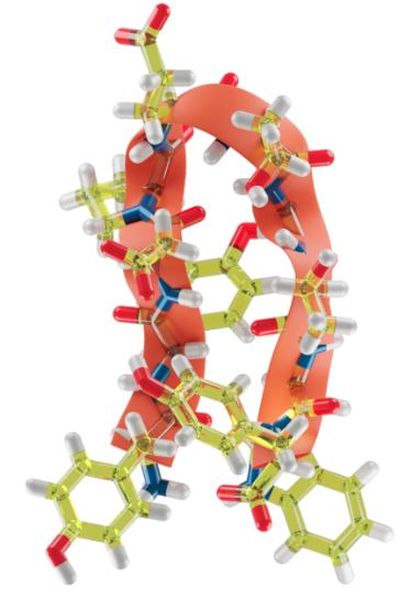
6c275e6bb9ae4f5b86479462b76b50de

Image credits: Narjes Ansari

Deep-TDA¶

We will use the folding of Chignolin protein as an example for the application of TPI-Deep-TDA as presented in TPI-Deep-TDA paper. As descriptors we will use the contacts between the \(\alpha\)-carbon of the protein chain.

[1]:

from mlcolvar.io import create_dataset_from_files
from mlcolvar.data import DictModule

filenames = [ "https://raw.githubusercontent.com/dhimanray/TPI_deepTDA/main/chignolin/training/folded/contacts_folded_25000",
              "https://raw.githubusercontent.com/dhimanray/TPI_deepTDA/main/chignolin/training/unfolded/contacts_unfolded_25000"]

n_states = len(filenames)

# load dataset
# here we only load part of the data to speed up the training, change stop to 25000 and stride to 1 to use them all for better results
dataset, df = create_dataset_from_files(filenames,
                                        create_labels=True,
                                        return_dataframe=True,
                                        filter_args={'regex':'cont' }, # select distances between heavy atoms
                                        stop=10000,
                                        stride=2)

datamodule = DictModule(dataset,lengths=[0.8,0.2])

/home/etrizio@iit.local/Bin/miniconda3/envs/mlcvs_test/lib/python3.10/site-packages/tqdm/auto.py:22: TqdmWarning: IProgress not found. Please update jupyter and ipywidgets. See https://ipywidgets.readthedocs.io/en/stable/user_install.html
  from .autonotebook import tqdm as notebook_tqdm

Class 0 dataframe shape:  (5000, 47)
Class 1 dataframe shape:  (5000, 47)

 - Loaded dataframe (10000, 47): ['cont1', 'cont2', 'cont3', 'cont4', 'cont5', 'cont6', 'cont7', 'cont8', 'cont9', 'cont10', 'cont11', 'cont12', 'cont13', 'cont14', 'cont15', 'cont16', 'cont17', 'cont18', 'cont19', 'cont20', 'cont21', 'cont22', 'cont23', 'cont24', 'cont25', 'cont26', 'cont27', 'cont28', 'cont29', 'cont30', 'cont31', 'cont32', 'cont33', 'cont34', 'cont35', 'cont36', 'cont37', 'cont38', 'cont39', 'cont40', 'cont41', 'cont42', 'cont43', 'cont44', 'cont45', 'walker', 'labels']
 - Descriptors (10000, 45): ['cont1', 'cont2', 'cont3', 'cont4', 'cont5', 'cont6', 'cont7', 'cont8', 'cont9', 'cont10', 'cont11', 'cont12', 'cont13', 'cont14', 'cont15', 'cont16', 'cont17', 'cont18', 'cont19', 'cont20', 'cont21', 'cont22', 'cont23', 'cont24', 'cont25', 'cont26', 'cont27', 'cont28', 'cont29', 'cont30', 'cont31', 'cont32', 'cont33', 'cont34', 'cont35', 'cont36', 'cont37', 'cont38', 'cont39', 'cont40', 'cont41', 'cont42', 'cont43', 'cont44', 'cont45']

Model¶

Here we use as target a series of three consecutive Gaussians, the second one will be broader as it is related to the TPE data

[2]:

from mlcolvar.cvs import DeepTDA

n_cvs = 1
target_centers = [-7,7]
target_sigmas = [0.2, 0.2]
nn_layers = [45,24,12,1]
# MODEL
model = DeepTDA(n_states=n_states, n_cvs=1,target_centers=target_centers, target_sigmas=target_sigmas, model=nn_layers)

We initialize the lightining.Trainer and Fit the model.

[5]:

from mlcolvar.utils.trainer import MetricsCallback

# define callbacks
metrics = MetricsCallback()

# define trainer
# for better results we can also increase the number of epochs or use a early_stopping
trainer = lightning.Trainer(callbacks=[metrics],
                     max_epochs=500, logger=None, enable_checkpointing=False)

# fit
trainer.fit( model, datamodule )

GPU available: True (cuda), used: True
TPU available: False, using: 0 TPU cores
IPU available: False, using: 0 IPUs
HPU available: False, using: 0 HPUs
Missing logger folder: /home/etrizio@iit.local/Bin/dev/mlcolvar/docs/notebooks/examples/lightning_logs
LOCAL_RANK: 0 - CUDA_VISIBLE_DEVICES: [0]

  | Name    | Type          | Params | In sizes | Out sizes
-----------------------------------------------------------------
0 | loss_fn | TDALoss       | 0      | ?        | ?
1 | norm_in | Normalization | 0      | [45]     | [45]
2 | nn      | FeedForward   | 1.4 K  | [45]     | [1]
-----------------------------------------------------------------
1.4 K     Trainable params
0         Non-trainable params
1.4 K     Total params
0.006     Total estimated model params size (MB)

/home/etrizio@iit.local/Bin/miniconda3/envs/mlcvs_test/lib/python3.10/site-packages/lightning/pytorch/loops/fit_loop.py:280: PossibleUserWarning: The number of training batches (1) is smaller than the logging interval Trainer(log_every_n_steps=50). Set a lower value for log_every_n_steps if you want to see logs for the training epoch.
  rank_zero_warn(

Epoch 499: 100%|██████████| 1/1 [00:00<00:00, 22.68it/s, v_num=0]

`Trainer.fit` stopped: `max_epochs=500` reached.

Epoch 499: 100%|██████████| 1/1 [00:00<00:00, 21.80it/s, v_num=0]

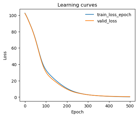
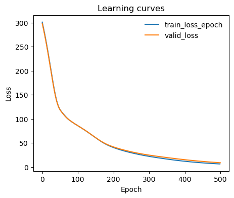
Learning curve

[6]:

from mlcolvar.utils.plot import plot_metrics

ax = plot_metrics(metrics.metrics,
                  keys=['train_loss_epoch','valid_loss'],
                  #linestyles=['-.','-'], colors=['fessa1','fessa5'],
                  yscale='linear')

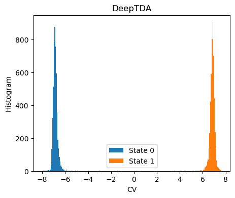
../../_images/notebooks_examples_ex_TPI-DeepTDA_14_0.png

Analysis of the CV¶

The histogram of the training data along th CVs should match the target distribution

[7]:

fig,ax = plt.subplots( 1, 1, figsize=(5,4) )

X = dataset[:]['data']
Y = dataset[:]['labels']

with torch.no_grad():
    s = model(torch.Tensor(X)).numpy()

for i in range(n_states):
    s_red = s[torch.nonzero(Y==i, as_tuple=True)]
    ax.hist(s_red[:,0],bins=100, label=f'State {i}')

ax.set_xlabel(f'CV')
ax.set_ylabel('Histogram')
ax.set_title('DeepTDA')
plt.legend()
plt.show()

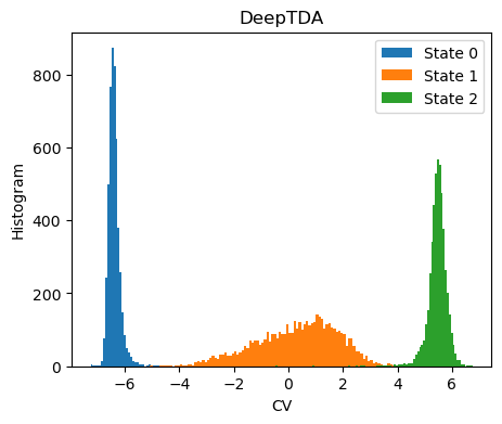
../../_images/notebooks_examples_ex_TPI-DeepTDA_17_0.png

Transition State Informed Deep-TDA (TPI-DeepTDA)¶

We will now try to imporve our CV using the TPI-Deep-TDA method, as presented in TPI-Deep-TDA paper. As descriptors we will again use the contacts between the \(\alpha\)-carbon of the protein chain. The data from the trasition path ensemble was collected by running a series of OPES-Flooding simualtions biasing a Deep-TDA CV as the one trained above.

[8]:

from mlcolvar.io import create_dataset_from_files
from mlcolvar.data import DictModule

filenames = [ "https://raw.githubusercontent.com/dhimanray/TPI_deepTDA/main/chignolin/training/folded/contacts_folded_25000",
              "https://raw.githubusercontent.com/dhimanray/TPI_deepTDA/main/chignolin/training/flooding/Contact_CV/contacts_ts_data",
              "https://raw.githubusercontent.com/dhimanray/TPI_deepTDA/main/chignolin/training/unfolded/contacts_unfolded_25000"]

n_states = len(filenames)

# load dataset
# here we only load part of the data to speed up the training, change stop to 25000 and stride to 1 to use them all for better results
dataset, df = create_dataset_from_files(filenames,
                                        create_labels=True,
                                        return_dataframe=True,
                                        filter_args={'regex':'cont' }, # select distances between heavy atoms
                                        stop=10000,
                                        stride=2)

datamodule = DictModule(dataset,lengths=[0.8,0.2])

Class 0 dataframe shape:  (5000, 47)
Class 1 dataframe shape:  (5000, 47)
Class 2 dataframe shape:  (5000, 47)

 - Loaded dataframe (15000, 47): ['cont1', 'cont2', 'cont3', 'cont4', 'cont5', 'cont6', 'cont7', 'cont8', 'cont9', 'cont10', 'cont11', 'cont12', 'cont13', 'cont14', 'cont15', 'cont16', 'cont17', 'cont18', 'cont19', 'cont20', 'cont21', 'cont22', 'cont23', 'cont24', 'cont25', 'cont26', 'cont27', 'cont28', 'cont29', 'cont30', 'cont31', 'cont32', 'cont33', 'cont34', 'cont35', 'cont36', 'cont37', 'cont38', 'cont39', 'cont40', 'cont41', 'cont42', 'cont43', 'cont44', 'cont45', 'walker', 'labels']
 - Descriptors (15000, 45): ['cont1', 'cont2', 'cont3', 'cont4', 'cont5', 'cont6', 'cont7', 'cont8', 'cont9', 'cont10', 'cont11', 'cont12', 'cont13', 'cont14', 'cont15', 'cont16', 'cont17', 'cont18', 'cont19', 'cont20', 'cont21', 'cont22', 'cont23', 'cont24', 'cont25', 'cont26', 'cont27', 'cont28', 'cont29', 'cont30', 'cont31', 'cont32', 'cont33', 'cont34', 'cont35', 'cont36', 'cont37', 'cont38', 'cont39', 'cont40', 'cont41', 'cont42', 'cont43', 'cont44', 'cont45']