Using mlcolvar with graph neural networks (GNNs)
![]()
Prerequisites:
Most of the workings of the library are the same using standard feed-forward-nn-based machine-learning CVs or GNN-based ones. Thus, it is recommended to first go through the basic tutorials for the standard scenario before moving to this tutorial.
Reference papers:
Author: Enrico Trizio
NOTE: For a more advanced usage of GNN models, allowing for better performance and lower computational costs in some scenarios, also check the tutorial on truncated GNNs.
Colab setup
[ ]:
# Colab setup
import os

if os.getenv("COLAB_RELEASE_TAG"):
    import subprocess
    subprocess.run('wget https://raw.githubusercontent.com/luigibonati/mlcolvar/main/colab_setup.sh', shell=True)
    cmd = subprocess.run('bash colab_setup.sh TUTORIAL', shell=True, stdout=subprocess.PIPE)
    print(cmd.stdout.decode('utf-8'))
Overview
Feed-Forward-based CVs vs GNN-based CVs
The default setting of mlcolvar is to represent the CVs as the output nodes of Feed-Forward Neural Networks (FFNNs or NNs, for simplicity) which take as input a set of physical descriptors (e.g., distances, angles, etc.). The code is thus designed to reflect this choice, with the default values of the classes set to intilialize the CV model in this framework, which is the most diffused for the time being in the field of machine-learning CVs and suits the needs of most users.
However, recently a different approach have been proposed, in which the CVs are represented as Graph Neural Networks (GNNs) which directly take as input the Cartesian coordinates of the atoms in the studied system and return the CV space after a node-pooling operation on the output layer. This approach is thus descriptor-free and goes in the direcion of a more automated way of desgining CVs. Unfortunately, it typically comes at a higher computational cost (i.e., slower training and evaluation fo the CV) and the underlying codebase is more complex (i.e., more complex models and data format.)
In this tutorial, we show how GNN models can be used within mlcolvar to build CVs using the implemented CV methods.
NOTE: the GNN-based require a specific interface for PLUMED, in which the graph is built in PLUMED on-the-fly. Updated source files for such interfaces and more info are available in the mlcovlar/plumed_interfaces folder.
Outline
Typically, the process of constructing a GNN-based CV requires the following ingredients;
A dataset of attributed connected graphs (nodes and edges), which are constructed from the atomic positions. The parameters of the dataset can also be used to initialize the model.
A GNN-model to represent the CV. Different architectures can be used in this regard.
A CV method and the associated loss function. These are all the methods implemented for standard machine-learning CVs, except for those based on autoencoders.
Load data
The input of GNN models are attributed and connected graphs, in which nodes (representing the atoms, in our case) are connected by edges (the lines of the graph). Nodes and edges are then assigned with scalar and, eventually, vector features that are then processed through the layers of the GNN.
In the context of GNN-CVs, such graphs most likely are created directly from the atomic coordinates from a trajectory file and the connectivity between the nodes is determined according to a radial cutoff.
In some cases, graphs can be built focusing the attention on a subset of the whole system, e.g., a molecule on a surface, but still keeping into account the interaction with the environment, e.g., the surface. In this case, only the nodes from the system_selection will be used for the final pooling, whereas the nodes from the enviroment_selection will be used only to update the information through the layers. Moreover, to reduce the computational costs, only the atoms closer to the
system_selection atoms will be included in the graphs, according to the set cutoff and a buffer value to ensure stability and continuity. For example, this setup is useful when treating solvent or surface interactions.
To make this process easier, in mlcolvar there is an util function to do this under-the-hood: create_dataset_from_trajectories, which is analogous to the create_dataset_from_files used with descriptors.
The loading process is built on the external library `MDTraj <https://www.mdtraj.org/>`__, which can natively load most common trajectory+topology format used in biophysics. One advantage of MDTraj, is that it comes with a simple and user friendly syntax for atom selection, which can be used also here.
For applications not related to biological system (e.g., solids, surfaces, molecules), we support the use of the .xyz file format. In this case, a topology pdb file is created using ase so that the convenient MDTraj selection syntax can be used. The generated pdb file can also be used as a topolgy file when running the simualtions in PLUMED.
Here, as an example, we load some data about the state A and B of Alanine Dipeptide.
[ ]:
from mlcolvar.data import DictModule
from mlcolvar.io import create_dataset_from_trajectories

# loading arguments
# same as to laod_dataframe
load_args = [{'start' : 0, 'stop' : 10000, 'stride' : 5},
               {'start' : 0, 'stop' : 10000, 'stride' : 5}]

# create dataset
dataset = create_dataset_from_trajectories(
    trajectories=["alad_A.trr",
                  "alad_B.trr"],
    topologies="alad.gro",
    folder="data/alanine_gnn",
    cutoff=10.0,  # Angstrom
    system_selection='all and not type H',
    show_progress=False,
    load_args=load_args,
    lengths_conversion=10.0, # MDTraj uses nm by default, we use Angstroms
    )
print('Dataset info:\n', dataset, end="\n\n")

# load dataset into a DictModule
datamodule = DictModule(dataset=dataset)
print('Datamodule info:\n', datamodule)
/home/etrizio@iit.local/Bin/dev/mlcolvar/mlcolvar/data/graph/utils.py:64: UserWarning: To copy construct from a tensor, it is recommended to use sourceTensor.clone().detach() or sourceTensor.clone().detach().requires_grad_(True), rather than torch.tensor(sourceTensor).
  graph_labels = torch.tensor( config.graph_labels, dtype=torch.get_default_dtype() )   if config.graph_labels is not None else None
Dataset info:
 DictDataset( "data_list": 4000,
            metadata={"atomic_numbers": [6, 7, 8],
                      "cutoff": 10.0,
                      "buffer": 0.0,
                      "used_idx": tensor([0, 1, 2, 3, 4, 5, 6, 7, 8, 9]),
                      "used_names": [ACE1-CH3, ACE1-C, ACE1-O, ALA2-N, ALA2-CA, ALA2-CB, ALA2-C, ALA2-O, NME3-N, NME3-C],
                      "data_type": graphs } )

Datamodule info:
 DictModule(dataset -> DictDataset( "data_list": 4000,
            metadata={"atomic_numbers": [6, 7, 8],
                      "cutoff": 10.0,
                      "buffer": 0.0,
                      "used_idx": tensor([0, 1, 2, 3, 4, 5, 6, 7, 8, 9]),
                      "used_names": [ACE1-CH3, ACE1-C, ACE1-O, ALA2-N, ALA2-CA, ALA2-CB, ALA2-C, ALA2-O, NME3-N, NME3-C],
                      "data_type": graphs } ),
             train_loader -> DictLoader(length=0.8, batch_size=4000, shuffle=True),
             valid_loader -> DictLoader(length=0.2, batch_size=4000, shuffle=True))
The built graphs are then stored as torch_geometric.Data objects into the usual DictDataset with the information about each graph entry (e.g., nodes positons, edges, weights, elabels etc.) under the key data_list and the common information for all the graphs (e.g., map from types to chemical species, cutoff) in the metadata attribute dictionary.
[3]:
print('Example of a graph entry:\n', dataset['data_list'][0], end='\n\n')
print('Dataset metadata:\n', dataset.metadata)
Example of a graph entry:
 Data(edge_index=[2, 90], shifts=[90, 3], unit_shifts=[90, 3], positions=[10, 3], cell=[3, 3], node_attrs=[10, 3], graph_labels=[1, 1], n_system=[1, 1], n_env=[1, 1], system_masks=[10, 1], weight=1.0, names_idx=[10])

Dataset metadata:
 {'atomic_numbers': [6, 7, 8], 'cutoff': 10.0, 'buffer': 0.0, 'used_idx': tensor([0, 1, 2, 3, 4, 5, 6, 7, 8, 9]), 'used_names': [ACE1-CH3, ACE1-C, ACE1-O, ALA2-N, ALA2-CA, ALA2-CB, ALA2-C, ALA2-O, NME3-N, NME3-C], 'data_type': 'graphs'}
Initializing the GNN model
At variance with the procedure with FFNNs, here the model is initialized outside the CV class, to which is then passed only later as an input. GNN architectures are indeed much more complex than FFNNs and have many parameters that can be set. In addition, when introducing GNN models into the code, we maintained the standard CVs as the default, which still covers most of the users.
Here, for example, we initialize a SchNetModel. Many other architectures are available in `pytorch_geometric <https://pytorch-geometric.readthedocs.io/en/latest/>`__ and can be readily adapted to this library.
As the input graph are built with the dataset and then processed in the GNN-model, we recommend initializing the model passing a dataset to the dataset_for_initialization keyword. This way, the values stored in the dataset.metadata (e.g., cutoff, atomic_numbers, buffer) will be infered from the dataset and registered in the model. This avoids possible mismatches and errors between the graphs in the training dataset, the model architecture and the graphs built in PLUMED during
the simulations (see the mlcovlar/plumed_interfaces folder).
Nonetheless, the cutoff, atomic_numbers and buffer variables can also be set manually setting dataset_for_initialization=None at you own risk.
[4]:
from mlcolvar.core.nn.graph.schnet import SchNetModel

gnn_model = SchNetModel(n_out=1,
                        dataset_for_initialization=dataset,
                        pooling_operation="mean",
                        n_bases=16,
                        n_layers=2,
                        n_filters=16,
                        n_hidden_channels=16,
                        w_out_after_pool=True,
                        aggr='mean'
                    )
Initializing CV class
The initalization of the CV class is almost identical to the standard case, with the only difference that we provide the initialized GNN object as model.
Here, for example, we use the DeepTDA CV.
[5]:
import torch
from mlcolvar.cvs import DeepTDA

# we can still set the options for the optimizer the usual way
# options for the BLOCKS of the cv are disabled when passing an external model
options = {'optimizer' : {'lr' : 1e-3},
           'lr_scheduler': {
            'scheduler': torch.optim.lr_scheduler.ExponentialLR,
            'gamma': 0.9999}
        }

model = DeepTDA(n_states=2,
                n_cvs=1,
                target_centers=[-7, 7],
                target_sigmas=[0.2, 0.2],
                model=gnn_model)
/home/etrizio@iit.local/Bin/miniconda3/envs/graph_mlcolvar_test_2.5/lib/python3.9/site-packages/lightning/pytorch/utilities/parsing.py:198: Attribute 'model' is an instance of `nn.Module` and is already saved during checkpointing. It is recommended to ignore them using `self.save_hyperparameters(ignore=['model'])`.
Training the CV
Here, everything works the same!
[ ]:
from lightning import Trainer
from mlcolvar.utils.trainer import MetricsCallback
from mlcolvar.utils.plot import plot_metrics
import matplotlib.pyplot as plt

# define callbacks
metrics = MetricsCallback()

# here the number of epochs is low for testing, you should increase it for applications
trainer = Trainer(
    callbacks=[metrics],
    logger=False,
    enable_checkpointing=False,
    max_epochs=5,
    enable_model_summary=False
)

trainer.fit(model, datamodule)
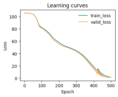
[7]:
fig, ax = plt.subplots(1,1,figsize=(4,3))
plot_metrics(metrics.metrics,
                  keys=['train_loss', 'valid_loss'],
                  colors=['fessa1', 'fessa5'],
                  yscale='linear',
                  ax = ax)
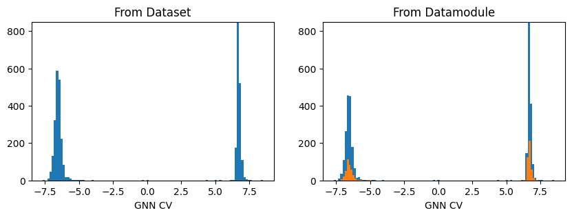
Testing the model
As the graph data are stored as torch_geometric.Data they need to be loaded using a loader object. For convenience, we implemented both in DictDataset and DictModule a method .get_graph_data to do it so that one can simply evaluate the model calling either:
model(dataset.get_graph_data())–> Returns the whole datasetmodel(datamodule.get_graph_data())–> Returns either the train or valid dataset
[8]:
fig, axs = plt.subplots(1,2, figsize=(10,3))

ax = axs[0]
out_graph = model(dataset.get_graph_inputs())
ax.hist(out_graph.detach().squeeze(), bins=100)
ax.set_title('From Dataset')
ax.set_xlabel('GNN CV')
ax.set_ylim(0,850)

ax = axs[1]
out_graph = model(datamodule.get_graph_inputs("train"))
ax.hist(out_graph.detach().squeeze(), bins=100)
out_graph = model(datamodule.get_graph_inputs("valid"))
ax.hist(out_graph.detach().squeeze(), bins=100)

ax.set_title('From Datamodule')
ax.set_xlabel('GNN CV')
ax.set_ylim(0,850)
plt.show()
Save the model to TorchScript
As for normal CVs, the frozen model can be saved to TorchScript suing the Lightning util to_torchscript using method=trace.
[9]:
traced_model = model.to_torchscript('gnn_model.pt', method='trace')

# we can also check the outputs coincide
torch.allclose(model(dataset.get_graph_inputs()), traced_model(dataset.get_graph_inputs()))
/home/etrizio@iit.local/Bin/dev/mlcolvar/mlcolvar/data/datamodule.py:341: UserWarning: Length of split at index 1 is 0. This might result in an empty dataset.
  warnings.warn(
[9]:
True
[ ]: