Stateinterpreter (characterizing DeepTICA states)

Reference paper: Novelli, Bonati, Pontil and Parrinello, JCTC (2023)

Prerequisite: LASSO tutorial.

Setup

# Colab setup
import os

if os.getenv("COLAB_RELEASE_TAG"):
    import subprocess
    subprocess.run('wget https://raw.githubusercontent.com/luigibonati/mlcolvar/main/colab_setup.sh', shell=True)
    cmd = subprocess.run('bash colab_setup.sh EXAMPLE', shell=True, stdout=subprocess.PIPE)
    print(cmd.stdout.decode('utf-8'))

# IMPORT PACKAGES
import torch
import lightning
import numpy as np
import matplotlib.pyplot as plt
import mlcolvar.utils.plot

# Set seed for reproducibility
torch.manual_seed(1)

/home/etrizio@iit.local/Bin/miniconda3/envs/mlcvs_test/lib/python3.10/site-packages/tqdm/auto.py:22: TqdmWarning: IProgress not found. Please update jupyter and ipywidgets. See https://ipywidgets.readthedocs.io/en/stable/user_install.html
  from .autonotebook import tqdm as notebook_tqdm

<torch._C.Generator at 0x7fbdc04804f0>

This is a short tutorial to interpret the states starting from the sign structure of the eigenfunctions of TICA, as done in this paper.

Load DeepTICA data

We will use the DeepTICA CVs trained for the alanine dipeptide, contained in the md-stateinterpreter repository.

from mlcolvar.io import create_dataset_from_files
from mlcolvar.data import DictModule

filenames = [ "https://github.com/luigibonati/md-stateinterpreter/raw/main/tutorials/alanine/COLVAR_DeepTICA" ]
# load dataset
dataset, df = create_dataset_from_files(filenames,
                                        filter_args={'regex':'d_' }, # select distances
                                        return_dataframe=True,
                                        index_col=0)

df

Class 0 dataframe shape:  (50001, 56)

 - Loaded dataframe (50001, 56): ['time', 'phi', 'psi', 'theta', 'xi', 'ene', 'd_2_5', 'd_2_6', 'd_2_7', 'd_2_9', 'd_2_11', 'd_2_15', 'd_2_16', 'd_2_17', 'd_2_19', 'd_5_6', 'd_5_7', 'd_5_9', 'd_5_11', 'd_5_15', 'd_5_16', 'd_5_17', 'd_5_19', 'd_6_7', 'd_6_9', 'd_6_11', 'd_6_15', 'd_6_16', 'd_6_17', 'd_6_19', 'd_7_9', 'd_7_11', 'd_7_15', 'd_7_16', 'd_7_17', 'd_7_19', 'd_9_11', 'd_9_15', 'd_9_16', 'd_9_17', 'd_9_19', 'd_11_15', 'd_11_16', 'd_11_17', 'd_11_19', 'd_15_16', 'd_15_17', 'd_15_19', 'd_16_17', 'd_16_19', 'd_17_19', 'ecv.ene', 'opes.bias', 'DeepTICA 1', 'DeepTICA 2', 'walker']
 - Descriptors (50001, 45): ['d_2_5', 'd_2_6', 'd_2_7', 'd_2_9', 'd_2_11', 'd_2_15', 'd_2_16', 'd_2_17', 'd_2_19', 'd_5_6', 'd_5_7', 'd_5_9', 'd_5_11', 'd_5_15', 'd_5_16', 'd_5_17', 'd_5_19', 'd_6_7', 'd_6_9', 'd_6_11', 'd_6_15', 'd_6_16', 'd_6_17', 'd_6_19', 'd_7_9', 'd_7_11', 'd_7_15', 'd_7_16', 'd_7_17', 'd_7_19', 'd_9_11', 'd_9_15', 'd_9_16', 'd_9_17', 'd_9_19', 'd_11_15', 'd_11_16', 'd_11_17', 'd_11_19', 'd_15_16', 'd_15_17', 'd_15_19', 'd_16_17', 'd_16_19', 'd_17_19']

	time	phi	psi	theta	xi	ene	d_2_5	d_2_6	d_2_7	d_2_9	...	d_15_17	d_15_19	d_16_17	d_16_19	d_17_19	ecv.ene	opes.bias	DeepTICA 1	DeepTICA 2	walker
0	0.0	-2.36867	2.64432	-0.202258	0.048056	-41.45820	0.152064	0.233505	0.241173	0.379827	...	0.130073	0.244001	0.227324	0.281913	0.148169	-41.45820	0.000000	0.884022	0.697792	0
1	1.0	-1.81603	2.26247	0.155789	-0.162735	-34.46170	0.154673	0.238446	0.246100	0.392822	...	0.130751	0.248974	0.224416	0.287066	0.149815	-34.46170	0.000000	0.904663	0.441770	0
2	2.0	-1.96164	2.52240	-0.071315	0.419557	-22.81000	0.153296	0.248231	0.245643	0.384574	...	0.133494	0.240812	0.219853	0.267548	0.146985	-22.81000	0.000000	0.901740	0.715535	0
3	3.0	-1.55273	2.61161	-0.073188	-0.322301	-19.42730	0.146842	0.233290	0.238608	0.375124	...	0.133732	0.243859	0.218035	0.273935	0.141663	-19.42730	0.000000	0.889557	0.327383	0
4	4.0	-1.43251	1.05203	0.210149	-0.033460	-31.27380	0.150544	0.238910	0.240522	0.374435	...	0.135397	0.254622	0.223741	0.285824	0.149050	-31.27380	0.000000	0.895487	-0.841115	0
...	...	...	...	...	...	...	...	...	...	...	...	...	...	...	...	...	...	...	...	...	...
49996	49996.0	-2.71024	3.09736	-0.278662	-0.145443	-17.50420	0.150316	0.237027	0.236800	0.371655	...	0.133984	0.245352	0.224751	0.283270	0.138847	-17.50420	1.543530	0.870904	0.345046	0
49997	49997.0	-2.73993	-3.07790	-0.066902	-0.030009	-9.98505	0.160066	0.240604	0.251294	0.387740	...	0.131298	0.245222	0.229207	0.287379	0.149105	-9.98505	0.983428	0.880671	0.498947	0
49998	49998.0	-1.79181	2.41757	0.454768	0.175903	28.20660	0.144505	0.220241	0.251352	0.389548	...	0.136430	0.243374	0.227492	0.275568	0.144445	28.20660	-14.739900	0.936590	0.497335	0
49999	49999.0	-2.25492	2.65134	-0.023274	0.166437	-31.68510	0.146304	0.232403	0.241591	0.381665	...	0.133528	0.245209	0.224884	0.281453	0.144545	-31.68510	1.717750	0.890656	0.782703	0
50000	50000.0	-1.30765	1.08041	-0.120033	0.027040	-20.90940	0.156149	0.247190	0.243012	0.387217	...	0.137467	0.249259	0.231183	0.290996	0.142807	-20.90940	1.633530	0.892738	-0.800826	0

50001 rows × 56 columns

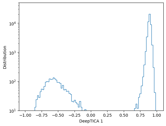
Lasso classifier (2 states)

If we look at the distribution of DeepTICA 1 we see that it identifies two states, which we can label accordingly:

fig, ax = plt.subplots()
ax.hist(df['DeepTICA 1'].values,bins=100,histtype='step')
ax.set_yscale('log')
ax.set_ylim(1e1,5e4)
ax.set_xlabel('DeepTICA 1')
ax.set_ylabel('Distribution')

Text(0, 0.5, 'Distribution')

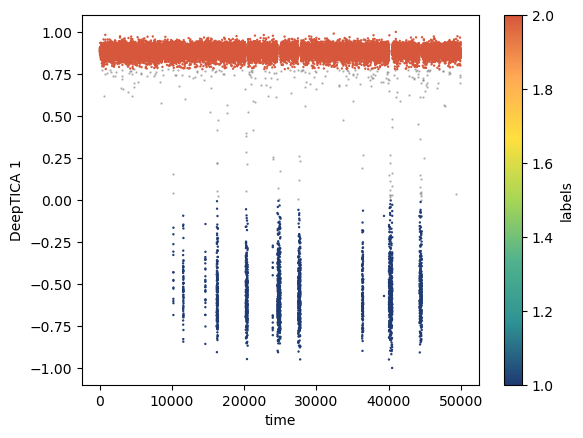
Create labels

labels = np.zeros(len(df))
labels[np.argwhere(df['DeepTICA 1'].values > 0.78)] = 2
labels[np.argwhere(df['DeepTICA 1'].values < -0.)] = 1
df['labels'] = labels

fig,ax = plt.subplots()
df[df['labels']==0].plot.scatter('time','DeepTICA 1',c='grey', s=0.5,alpha=0.5,ax=ax)
df[df['labels']!=0].plot.scatter('time','DeepTICA 1',c='labels', s=0.5,cmap='fessa',ax=ax)

<AxesSubplot:xlabel='time', ylabel='DeepTICA 1'>

Create dataset with angles or distances

from mlcolvar.data import DictDataset

sel = (df['labels'] != 0 )

descr_type = 'angles' #'distances'

if descr_type == 'angles':
    # get descriptors
    X = df[sel].filter(regex='phi|psi|xi|theta').values[::10]
    feat_names = df[sel].filter(regex='phi|psi|xi|theta').columns.values

    # convert to sine and cosine
    X = np.hstack((np.sin(X),np.cos(X)))
    feat_names = [f'sin_{i}' for i in feat_names]+[f'cos_{i}' for i in feat_names]

    # get labels
    y = df[sel]['labels'].values[::10]

elif descr_type == 'distances':
    # get descriptors
    X = df[sel].filter(regex='d_').values[::10]
    feat_names = df[sel].filter(regex='d_').columns.values

    # get labels
    y = df[sel]['labels'].values[::10]

# create dataset
dataset = DictDataset(dict(data=X,labels=y))
dataset.feature_names = feat_names
dataset

DictDataset( "data": [4976, 8], "labels": [4976] )

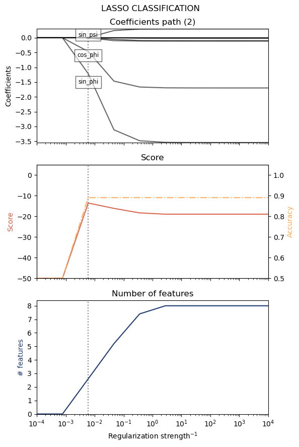
Perform classification

from mlcolvar.explain.lasso import lasso_classification

classifier, feats, coeffs = lasso_classification(dataset, Cs=10, plot=True)

======= LASSO results (2) ========
- Regularization : 0.00599484
- Score          : -13.58
- Accuracy       : 89.42%
- # features     : 3

Features:
(1) sin_phi      : -1.556827
(2) cos_phi      : -0.656852
(3) sin_psi      : 0.040250
==================================

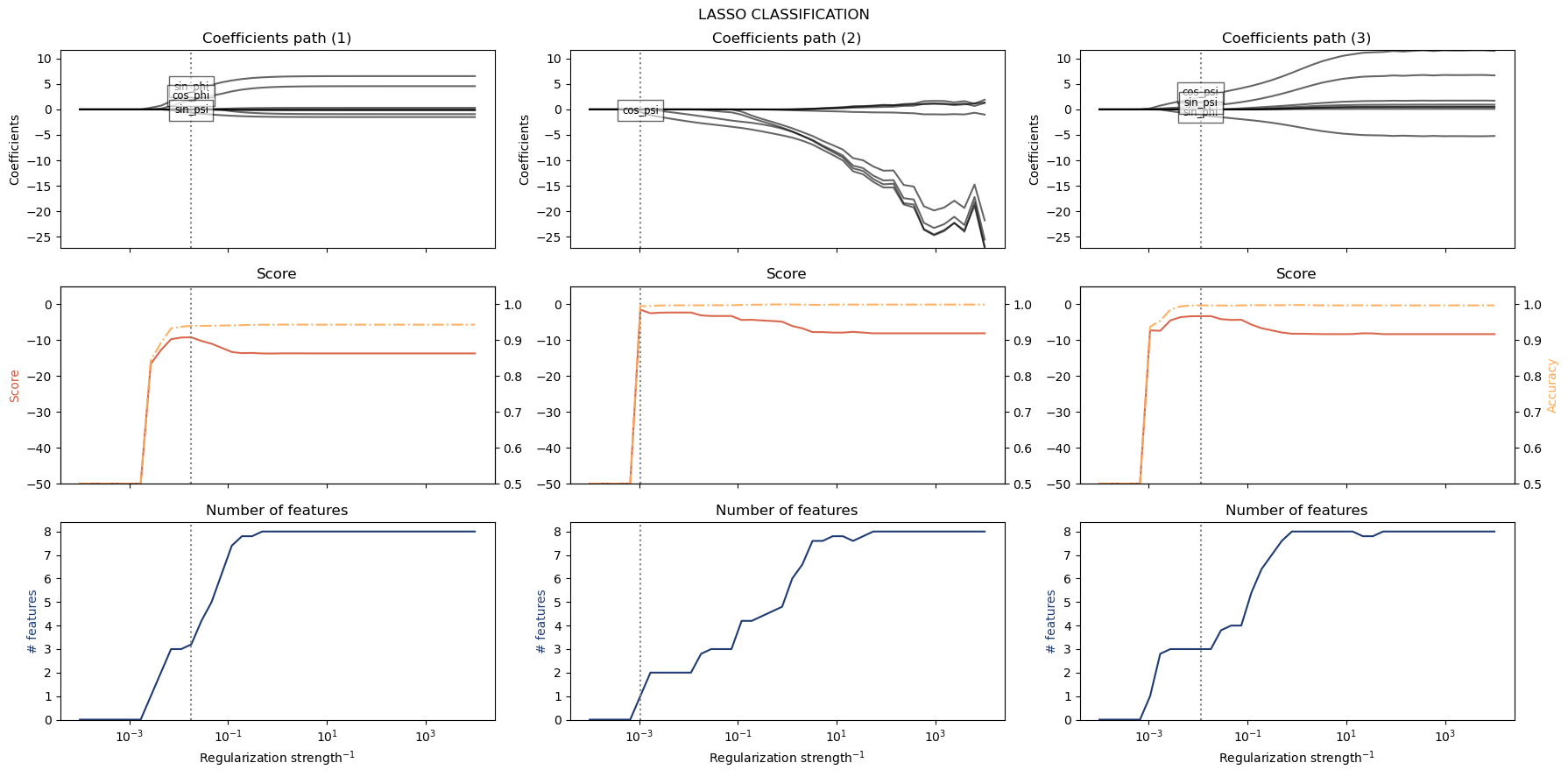
Lasso classifier (3 states, one vs rest)

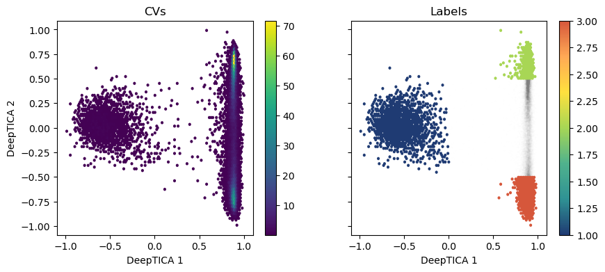
If we look instead at both DeepTICA 1 and DeepTICA 2 variables, we see that they identify three distinct states. We can then interpret them using a classifier for each state (‘one vs rest’) which returns the features that distinguish that state from all the others.

fig,axs = plt.subplots(1,2,figsize=(10,4),sharex=True,sharey=True)

ax = axs[0]
pp = ax.hexbin(df['DeepTICA 1'],df['DeepTICA 2'], C = np.ones(len(df)), reduce_C_function = lambda x: np.sum(x)/10 )
plt.colorbar(pp,ax=ax)

ax = axs[1]

labels = np.zeros(len(df))
labels[np.argwhere( (df['DeepTICA 1'].values < 0) )] = 1
labels[np.argwhere( (df['DeepTICA 1'].values > 0.5) & (df['DeepTICA 2'].values > 0.5) )] = 2
labels[np.argwhere( (df['DeepTICA 1'].values > 0.5) & (df['DeepTICA 2'].values < -0.5) )] = 3
df['labels'] = labels

df[df['labels']==0].plot.scatter('DeepTICA 1','DeepTICA 2',c='grey', s=0.1,alpha=0.01,ax=ax)
df[df['labels'] != 0].plot.hexbin('DeepTICA 1','DeepTICA 2',C='labels', cmap='fessa',ax=ax)

titles = ['CVs','Labels']
for i,ax in enumerate(axs):
    ax.set_xlabel('DeepTICA 1')
    ax.set_ylabel('DeepTICA 2')
    ax.set_title(titles[i])

Create new dataset

from mlcolvar.data import DictDataset

sel = (df['labels'] != 0 )

descr_type = 'angles'#'distances' #

if descr_type == 'angles':
    # get descriptors
    X = df[sel].filter(regex='phi|psi|xi|theta').values[::10]
    feat_names = df[sel].filter(regex='phi|psi|xi|theta').columns.values

    # convert to sine and cosine
    X = np.hstack((np.sin(X),np.cos(X)))
    feat_names = [f'sin_{i}' for i in feat_names]+[f'cos_{i}' for i in feat_names]

    # get labels
    y = df[sel]['labels'].values[::10]

elif descr_type == 'distances':
    # get descriptors
    X = df[sel].filter(regex='d_').values[::10]
    feat_names = df[sel].filter(regex='d_').columns.values

    # get labels
    y = df[sel]['labels'].values[::10]

# create dataset
dataset = DictDataset(dict(data=X,labels=y))
dataset.feature_names = feat_names
dataset

DictDataset( "data": [3331, 8], "labels": [3331] )

Perform classification

classifier, feats, coeffs = lasso_classification(dataset, plot = False)

======= LASSO results (1) ========
- Regularization : 0.01804722
- Score          : -9.23
- Accuracy       : 93.77%
- # features     : 3

Features:
(1) sin_phi      : 3.842064
(2) cos_phi      : 2.095998
(3) sin_psi      : -0.727435
==================================

======= LASSO results (2) ========
- Regularization : 0.00106082
- Score          : -1.54
- Accuracy       : 99.46%
- # features     : 1

Features:
(1) cos_psi      : -0.836221
==================================

======= LASSO results (3) ========
- Regularization : 0.01125336
- Score          : -3.35
- Accuracy       : 99.65%
- # features     : 3

Features:
(1) cos_psi      : 2.700127
(2) sin_phi      : -1.191376
(3) sin_psi      : 0.681767
==================================

Plot

from mlcolvar.explain.lasso import plot_lasso_classification

plot_lasso_classification(classifier,feats,coeffs)