Deep-TDA: Deep Targeted Discriminant Analysis
Reference papers:
![]()
Introduction
The Deep Targeted Discriminant Analysis (DeepTDA) is a method for the supervised learning of discriminant-based collective variables (CVs) starting from information limited to the \(N_s\) metastable states only.
In DeepTDA a Neural Network (NN) is used to map a high-dimensional set of descriptors \(\mathbf{d}\), collected in the metastable states, into a low-dimensional CV space \(\mathbf{s}\). The NN is trained so that the data from each metastable state, when projected along the CV, are distributed according to a preassigned target in which the different states are well-defined. In the practice, this target is taken as a sum of \(N_s\) Gaussians, one for each state in the system.

The extension to the multi-case scenario is straightforward with DeepTDA. In general, given \(N_s\) states, on needs to define \((N_s -1)\) CVs to fully account for all the possible transitions between them. In DeepTDA these CVs are built imposing a target that is a linear superimposition of \(N_s\) multivariate Gaussians with diagonal covariances.
However, it often happens that the number of CVs can be reduced if the different states can only be visited in a precise order, i.e. in chemical reactions with stable intermidiates or with alternative and exclusive products from the same reagents. In this scenario DeepTDA allows to built one-dimensional CVs by simply imposing a target in which the ordering of the states is respected.
Optimization criterion
Each state \(k\) thus contributes two terms for each dimension \(\rho\) of the CVs space \(\mathbf{s}\) to the loss function which has to be minimized during the training of the model.
The term \(L^\mu_{k,\rho}\) enfroces the position of the center \(\mu\) of the distribution of data from state \(k\) along the dimension \(\rho\) to match the target one \(\mu^tg\). The second term \(L^\sigma_{k,\rho}\) does the same thing for the width of the distribution, defined as the standard deviation.
The total loss function is obtained by summing over the \(N_s\) states \(k\) and the \(N_d\) dimension \(\rho\) of the CVs space:
Where \(\alpha\) and \(\beta\) hyperparameters are used to balance the center and width contributions to the loss to roughly the same magnitude in the first stage of the training.
Choice of the target
Fast most-of-the-times recipe:
target_centers: The Gaussians associated to different metastable states should be placed in a way such that the distance with respect to other Gaussians is at least around 10/20 au. For example \(\mu_A =-7, \mu_B=7\)target_sigmas: Widths of the order of 0.2/0.5 should be fine most of the time.
Rationale behind : In order to get an effective DeepTDA CV the Gaussians associated to the different states must be:
Not too close to each other otherwise the there would not be enough space in between for the transition state (on which typically one has very limited information)
Not too far each other otherwise most of the CV space would require the NN to extrapolate rather than to interpolate from the provided data.
Not too narrow, besides being unphysical this would also lead to a very strong dependence on the atomic positions, which is better to be avoided in a biasing context as it would result in very strong forces
Not too wide, besides being unphysical this would also lead to a very weak dependence on the atomic positions, which is better to be avoided in a biasing context as it would result in very small forces
TPI-Deep-TDA
A further improvement over Deep-TDA is its Transition Path Informed (TPI) version. This method allows to refine in a second moment a Deep-TDA CV by including in the training set also data from the Transition Path Ensemble (TPE) and treating them as a separate class (see the workflow below for a two state system). This in general both improves and speeds up the convergence of the simulations as it provides to the model also information between the metastable states.

In the practice, the TPE data are collected by trimming reactive trajectories which can be easily generated with the OPES-Flooding biasing scheme using a standard Deep-TDA CV. However, in principle, similar results could be achieved with different techniques (high T, metadynamics, Gambes..). The TPE is added to the Deep-TDA CV as a broader (\(\sigma_{TPE}\) = 1.0/2.0) state between the metastable ones, still ensuring a negligible overlap with them.
Setup
[1]:
# Colab setup
import os

if os.getenv("COLAB_RELEASE_TAG"):
    import subprocess
    subprocess.run('wget https://raw.githubusercontent.com/luigibonati/mlcolvar/main/colab_setup.sh', shell=True)
    cmd = subprocess.run('bash colab_setup.sh TUTORIAL', shell=True, stdout=subprocess.PIPE)
    print(cmd.stdout.decode('utf-8'))

# IMPORT PACKAGES
import torch
import lightning
import numpy as np
import matplotlib.pyplot as plt

# IMPORT HELPER FUNCTIONS
from mlcolvar.utils.plot import muller_brown_potential, plot_isolines_2D, plot_metrics

# Set seed for reproducibility
torch.manual_seed(42)
/home/etrizio@iit.local/Bin/miniconda3/envs/mlcvs_test/lib/python3.10/site-packages/tqdm/auto.py:22: TqdmWarning: IProgress not found. Please update jupyter and ipywidgets. See https://ipywidgets.readthedocs.io/en/stable/user_install.html
  from .autonotebook import tqdm as notebook_tqdm
[1]:
<torch._C.Generator at 0x7f6295c1c510>
Two states case
Load MD data
We will use the two-state Muller-Brown potential as first example using p.x and p.y as descriptors. To easily create a dataset we can use the util create_dataset_from_files and from that we initilize the lightning DictModule for the training.
[2]:
from mlcolvar.utils.io import create_dataset_from_files
from mlcolvar.data import DictModule

n_states = 2
filenames = [ f"data/muller-brown/unbiased/state-{i}/COLVAR" for i in range(n_states) ]

# load dataset
dataset, df = create_dataset_from_files(filenames,return_dataframe=True, filter_args={'regex':'p.x|p.y'})

# create datamodule for trainere
datamodule = DictModule(dataset,lengths=[0.8,0.2])
datamodule
Class 0 dataframe shape:  (2001, 13)
Class 1 dataframe shape:  (2001, 13)

 - Loaded dataframe (4002, 13): ['time', 'p.x', 'p.y', 'p.z', 'ene', 'pot.bias', 'pot.ene_bias', 'lwall.bias', 'lwall.force2', 'uwall.bias', 'uwall.force2', 'walker', 'labels']
 - Descriptors (4002, 2): ['p.x', 'p.y']
[2]:
DictModule(dataset -> DictDataset( "data": [4002, 2], "labels": [4002] ),
                     train_loader -> DictLoader(length=0.8, batch_size=0, shuffle=True),
                     valid_loader -> DictLoader(length=0.2, batch_size=0, shuffle=True))
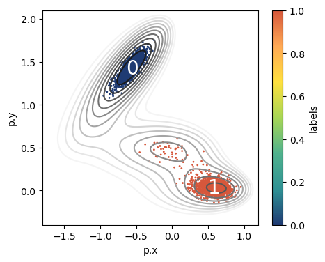
We can use the plot_isolines_2D util to have a quick sketch of the Muller-Brown potential.
[3]:
fig,ax = plt.subplots(figsize=(5,4),dpi=100)
# ploy MB isolines
plot_isolines_2D(muller_brown_potential,mode='contour',levels=np.linspace(0,24,12),ax=ax)
# plot points colored according to labels
df.plot.scatter('p.x','p.y',c='labels',s=1,cmap='fessa',ax=ax)
# draw state labels
for i in range(n_states):
    df_g = df.groupby('labels').mean()
    ax.text(x = df_g['p.x'].values[i]-0.075,
            y = df_g['p.y'].values[i]-0.075,
            s = str(i), size=20, color='white')
Model
We import the DeepTDA CV class and initialize it with the target parameters. Here as target we just use two Gaussian in one dimension.
[4]:
from mlcolvar.cvs import DeepTDA

# Parameters
n_cvs = 1
target_centers = [-7, 7]
target_sigmas = [0.2, 0.2]
nn_layers = [2,24,12,1]

# Initialize DeepTDA model
model = DeepTDA(n_states=n_states, n_cvs=1,target_centers=target_centers, target_sigmas=target_sigmas, layers=nn_layers)
We initialize the lightining.Trainer and Fit the model.
[5]:
from lightning.pytorch.callbacks.early_stopping import EarlyStopping
from mlcolvar.utils.trainer import MetricsCallback

# define callbacks
metrics = MetricsCallback()
early_stopping = EarlyStopping(monitor="valid_loss", mode='min', min_delta=1e-2, patience=20)

# define trainer
trainer = lightning.Trainer(callbacks=[metrics, early_stopping],
                     max_epochs=400, logger=None, enable_checkpointing=False)

# fit
trainer.fit( model, datamodule )
GPU available: True (cuda), used: True
TPU available: False, using: 0 TPU cores
IPU available: False, using: 0 IPUs
HPU available: False, using: 0 HPUs
LOCAL_RANK: 0 - CUDA_VISIBLE_DEVICES: [0]

  | Name    | Type          | Params | In sizes | Out sizes
-----------------------------------------------------------------
0 | loss_fn | TDALoss       | 0      | ?        | ?
1 | norm_in | Normalization | 0      | [2]      | [2]
2 | nn      | FeedForward   | 385    | [2]      | [1]
-----------------------------------------------------------------
385       Trainable params
0         Non-trainable params
385       Total params
0.002     Total estimated model params size (MB)
/home/etrizio@iit.local/Bin/miniconda3/envs/mlcvs_test/lib/python3.10/site-packages/lightning/pytorch/loops/fit_loop.py:280: PossibleUserWarning: The number of training batches (1) is smaller than the logging interval Trainer(log_every_n_steps=50). Set a lower value for log_every_n_steps if you want to see logs for the training epoch.
  rank_zero_warn(
Epoch 399: 100%|██████████| 1/1 [00:00<00:00, 28.42it/s, v_num=88]
`Trainer.fit` stopped: `max_epochs=400` reached.
Epoch 399: 100%|██████████| 1/1 [00:00<00:00, 27.02it/s, v_num=88]
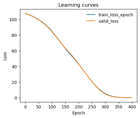
Learning curve
[6]:
ax = plot_metrics(metrics.metrics,
                  keys=['train_loss_epoch','valid_loss'],
                  #linestyles=['-.','-'], colors=['fessa1','fessa5'],
                  yscale='linear')
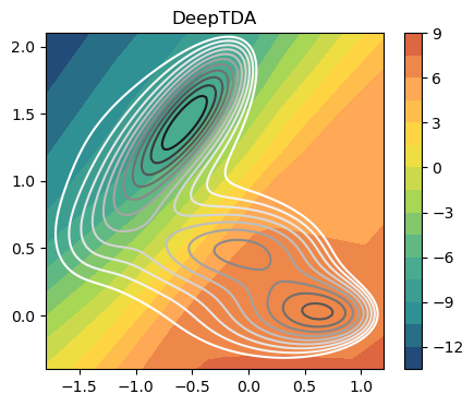
Analysis of the CV
The CV isolines should follow the underlying free energy landscape.
[7]:
fig,ax = plt.subplots( 1, 1, figsize=(5,4) )

plot_isolines_2D(muller_brown_potential,levels=np.linspace(0,24,12),mode='contour',ax=ax)
plot_isolines_2D(model, levels=15, ax=ax)
ax.set_title('DeepTDA')
plt.show()
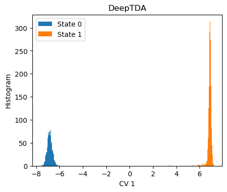
The histogram of the training points along the CV should match the target distribution.
[8]:
fig,ax = plt.subplots( 1, 1, figsize=(5,4) )

X = dataset[:]['data']
Y = dataset[:]['labels']

with torch.no_grad():
    s = model(torch.Tensor(X)).numpy()

for i in range(n_states):
    s_red = s[torch.nonzero(Y==i, as_tuple=True)]
    ax.hist(s_red[:,0],bins=100, label=f'State {i}')

ax.set_xlabel(f'CV {i}')
ax.set_ylabel('Histogram')
ax.set_title('DeepTDA')
plt.legend()
plt.show()
Multi-state case
We first start from the general approch (\(N_{d} = N_s - 1\)), training a two-dimensional DeepTDA CV for a \(N_s=3\) states system.
Load MD data
We will use a modified three-state Muller-Brown potential as multi-state example using p.x and p.y as descriptors.
[9]:
n_states = 3
filenames = [ f"data/muller-brown-3states/unbiased/state-{i}/COLVAR" for i in range(n_states) ]

# load dataset
dataset, df = create_dataset_from_files(filenames,return_dataframe=True, filter_args={'regex':'p.x|p.y'})

# create datamodule for trainere
datamodule = DictModule(dataset,lengths=[0.8,0.2])
datamodule
Class 0 dataframe shape:  (2001, 13)
Class 1 dataframe shape:  (2001, 13)
Class 2 dataframe shape:  (2001, 13)

 - Loaded dataframe (6003, 13): ['time', 'p.x', 'p.y', 'p.z', 'ene', 'pot.bias', 'pot.ene_bias', 'lwall.bias', 'lwall.force2', 'uwall.bias', 'uwall.force2', 'walker', 'labels']
 - Descriptors (6003, 2): ['p.x', 'p.y']
[9]:
DictModule(dataset -> DictDataset( "data": [6003, 2], "labels": [6003] ),
                     train_loader -> DictLoader(length=0.8, batch_size=0, shuffle=True),
                     valid_loader -> DictLoader(length=0.2, batch_size=0, shuffle=True))
[10]:
from mlcolvar.utils.plot import muller_brown_potential_three_states

fig,ax = plt.subplots(figsize=(5,4),dpi=100)
# ploy MB isolines
plot_isolines_2D(muller_brown_potential_three_states,mode='contour',levels=np.linspace(0,24,12),ax=ax)
# plot points colored according to labels
df.plot.scatter('p.x','p.y',c='labels',s=1,cmap='fessa',ax=ax)
# draw state labels
for i in range(n_states):
    df_g = df.groupby('labels').mean()
    ax.text(x = df_g['p.x'].values[i]-0.075,
            y = df_g['p.y'].values[i]-0.075,
            s = str(i), size=20, color='white')

Model
The same rules of thumb for the choice of the target can be applied also in the multi-dimensional CVs space. For the sake of simplicity we will place the three states at the verteces of an equilateral triangle.
[11]:
n_cvs = 2
# The targets should be two-dimensional
target_centers = [[-4, -5], # state 0 [cv_0.mu, cv_1.mu]
                  [ 0,  5],
                  [ 4, -5]]
target_sigmas = [[0.2, 0.2], # state 0 [cv_0.sigma, cv_1.sigma]
                 [0.2, 0.2],
                 [0.2, 0.2]]
nn_layers = [2,24,12,2]

# MODEL
model = DeepTDA(n_states=n_states,
                n_cvs=2,
                target_centers=target_centers,
                target_sigmas=target_sigmas,
                layers=nn_layers)
We initialize the lightining.Trainer and Fit the model.
[12]:
from lightning.pytorch.callbacks.early_stopping import EarlyStopping
from mlcolvar.utils.trainer import MetricsCallback

# define callbacks
metrics = MetricsCallback()
early_stopping = EarlyStopping(monitor="train_loss", mode='min', min_delta=1e-1, patience=20)

# define trainer
trainer = lightning.Trainer(callbacks=[metrics, early_stopping],
                     max_epochs=500, logger=None, enable_checkpointing=False)

# fit
trainer.fit( model, datamodule )
GPU available: True (cuda), used: True
TPU available: False, using: 0 TPU cores
IPU available: False, using: 0 IPUs
HPU available: False, using: 0 HPUs
LOCAL_RANK: 0 - CUDA_VISIBLE_DEVICES: [0]

  | Name    | Type          | Params | In sizes | Out sizes
-----------------------------------------------------------------
0 | loss_fn | TDALoss       | 0      | ?        | ?
1 | norm_in | Normalization | 0      | [2]      | [2]
2 | nn      | FeedForward   | 398    | [2]      | [2]
-----------------------------------------------------------------
398       Trainable params
0         Non-trainable params
398       Total params
0.002     Total estimated model params size (MB)
/home/etrizio@iit.local/Bin/miniconda3/envs/mlcvs_test/lib/python3.10/site-packages/lightning/pytorch/loops/fit_loop.py:280: PossibleUserWarning: The number of training batches (1) is smaller than the logging interval Trainer(log_every_n_steps=50). Set a lower value for log_every_n_steps if you want to see logs for the training epoch.
  rank_zero_warn(
Epoch 499: 100%|██████████| 1/1 [00:00<00:00, 26.63it/s, v_num=89]
`Trainer.fit` stopped: `max_epochs=500` reached.
Epoch 499: 100%|██████████| 1/1 [00:00<00:00, 24.60it/s, v_num=89]
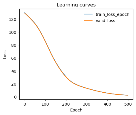
Learning curve
[13]:
ax = plot_metrics(metrics.metrics,
                  keys=['train_loss_epoch','valid_loss'],
                  #linestyles=['-.','-'], colors=['fessa1','fessa5'],
                  yscale='linear')
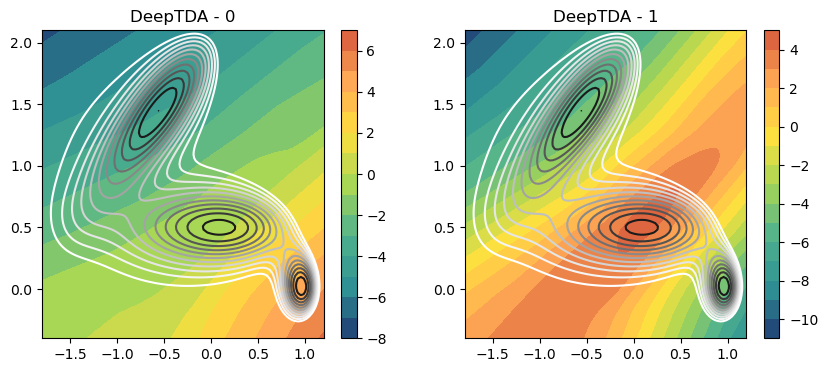
Analysis of the CV
Here the two CVs isolines should give us different informations!
[14]:
fig,axs = plt.subplots( 1, 2, figsize=(10,4) )
for i in range(2):
    ax = axs[i]
    plot_isolines_2D(muller_brown_potential_three_states,levels=np.linspace(0,24,12),mode='contour',ax=ax)
    plot_isolines_2D(model, component=i, levels=15, ax=ax)
    ax.set_title(f'DeepTDA - {i}')
plt.show()
The scatter plot of the training data in the CVs space should correspond to the verteces of the equilateral triangle we used as target.
[15]:
fig,ax = plt.subplots( 1, 1, figsize=(5,4) )

X = dataset[:]['data']
Y = dataset[:]['labels']

with torch.no_grad():
    s = model(torch.Tensor(X)).numpy()

for i in range(n_states):
    s_red = s[torch.nonzero(Y==i, as_tuple=True)]
    ax.scatter(s_red[:, 0], s_red[:,1], label=f'State {i}', alpha=0.5, s=10)

ax.set_xlabel(f'CV 0')
ax.set_ylabel('CV 2')
ax.set_title('DeepTDA')
plt.legend()
plt.show()

Multi-state reduced
We now exploit the fact that only \(S_0 \leftrightarrow S_1 \leftrightarrow S_2\) transitions are allowed to reduce the dimension of the DeepTDA CVs space to \(N_d = 1\) for a \(N_s=3\) states system.
Load MD data
We will use a modified three-state Muller-Brown potential as multi-state example using p.x and p.y as descriptors.
[16]:
n_states = 3
filenames = [ f"data/muller-brown-3states/unbiased/state-{i}/COLVAR" for i in range(n_states) ]

# load dataset
dataset, df = create_dataset_from_files(filenames,return_dataframe=True, filter_args={'regex':'p.x|p.y'})

# create datamodule for trainere
datamodule = DictModule(dataset,lengths=[0.8,0.2])
datamodule
Class 0 dataframe shape:  (2001, 13)
Class 1 dataframe shape:  (2001, 13)
Class 2 dataframe shape:  (2001, 13)

 - Loaded dataframe (6003, 13): ['time', 'p.x', 'p.y', 'p.z', 'ene', 'pot.bias', 'pot.ene_bias', 'lwall.bias', 'lwall.force2', 'uwall.bias', 'uwall.force2', 'walker', 'labels']
 - Descriptors (6003, 2): ['p.x', 'p.y']
[16]:
DictModule(dataset -> DictDataset( "data": [6003, 2], "labels": [6003] ),
                     train_loader -> DictLoader(length=0.8, batch_size=0, shuffle=True),
                     valid_loader -> DictLoader(length=0.2, batch_size=0, shuffle=True))
[17]:
fig,ax = plt.subplots(figsize=(5,4),dpi=100)
# ploy MB isolines
plot_isolines_2D(muller_brown_potential_three_states,mode='contour',levels=np.linspace(0,24,12),ax=ax)
# plot points colored according to labels
df.plot.scatter('p.x','p.y',c='labels',s=1,cmap='fessa',ax=ax)
# draw state labels
for i in range(n_states):
    df_g = df.groupby('labels').mean()
    ax.text(x = df_g['p.x'].values[i]-0.075,
            y = df_g['p.y'].values[i]-0.075,
            s = str(i), size=20, color='white')

Model
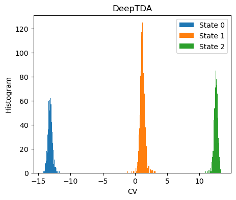
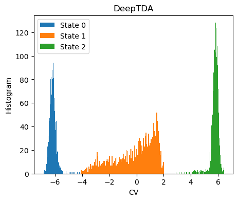
Here we use as target a series of three consecutive Gaussians on a single CV dimension
[18]:
n_cvs = 1
target_centers = [-14,0,14]
target_sigmas = [0.2, 0.2, 0.2]
nn_layers = [2,24,12,1]
# MODEL
model = DeepTDA(n_states=n_states, n_cvs=1,target_centers=target_centers, target_sigmas=target_sigmas, layers=nn_layers)
We initialize the lightining.Trainer and Fit the model.
[19]:
from lightning.pytorch.callbacks.early_stopping import EarlyStopping
from mlcolvar.utils.trainer import MetricsCallback

# define callbacks
metrics = MetricsCallback()
early_stopping = EarlyStopping(monitor="train_loss", mode='min', min_delta=1e-2, patience=20)

# define trainer
trainer = lightning.Trainer(callbacks=[metrics, early_stopping],
                     max_epochs=600, logger=None, enable_checkpointing=False)

# fit
trainer.fit( model, datamodule )
GPU available: True (cuda), used: True
TPU available: False, using: 0 TPU cores
IPU available: False, using: 0 IPUs
HPU available: False, using: 0 HPUs
LOCAL_RANK: 0 - CUDA_VISIBLE_DEVICES: [0]

  | Name    | Type          | Params | In sizes | Out sizes
-----------------------------------------------------------------
0 | loss_fn | TDALoss       | 0      | ?        | ?
1 | norm_in | Normalization | 0      | [2]      | [2]
2 | nn      | FeedForward   | 385    | [2]      | [1]
-----------------------------------------------------------------
385       Trainable params
0         Non-trainable params
385       Total params
0.002     Total estimated model params size (MB)
/home/etrizio@iit.local/Bin/miniconda3/envs/mlcvs_test/lib/python3.10/site-packages/lightning/pytorch/loops/fit_loop.py:280: PossibleUserWarning: The number of training batches (1) is smaller than the logging interval Trainer(log_every_n_steps=50). Set a lower value for log_every_n_steps if you want to see logs for the training epoch.
  rank_zero_warn(
Epoch 599: 100%|██████████| 1/1 [00:00<00:00, 26.48it/s, v_num=90]
`Trainer.fit` stopped: `max_epochs=600` reached.
Epoch 599: 100%|██████████| 1/1 [00:00<00:00, 25.13it/s, v_num=90]
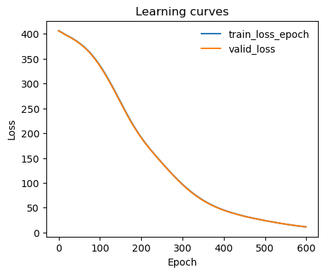
Learning curve
[20]:
ax = plot_metrics(metrics.metrics,
                  keys=['train_loss_epoch','valid_loss'],
                  #linestyles=['-.','-'], colors=['fessa1','fessa5'],
                  yscale='linear')
Analysis of the CV
Here the isolines of a single CVs should be able to follow the free energy ladscape across all the three states
[21]:
fig,ax = plt.subplots( 1, 1, figsize=(5,4) )

plot_isolines_2D(muller_brown_potential_three_states,levels=np.linspace(0,24,12),mode='contour',ax=ax)
plot_isolines_2D(model, levels=15, ax=ax)
ax.set_title('DeepTDA')
plt.show()

The histogram of the training data along th CVs should match the target distribution
[22]:
fig,ax = plt.subplots( 1, 1, figsize=(5,4) )

X = dataset[:]['data']
Y = dataset[:]['labels']

with torch.no_grad():
    s = model(torch.Tensor(X)).numpy()

for i in range(n_states):
    s_red = s[torch.nonzero(Y==i, as_tuple=True)]
    ax.hist(s_red[:,0],bins=100, label=f'State {i}')

ax.set_xlabel(f'CV')
ax.set_ylabel('Histogram')
ax.set_title('DeepTDA')
plt.legend()
plt.show()
TPI-Deep-TDA
We now try to refine our CV by including in the training set data from the transition path ensemble as a third state between the metastable ones.
Load data
We will use the two-state Muller-Brown potential using p.x and p.y as descriptors as an example for the application of TPI-Deep-TDA, as presented in TPI-Deep-TDA paper.
The data from the transition state region have been collected by running a series of OPES-Flooding simulations along Deep-TDA CV.
[24]:
from mlcolvar.utils.io import create_dataset_from_files
from mlcolvar.data import DictModule

filenames = [ "data/muller-brown/unbiased/state-0/COLVAR",
              "data/muller-brown/biased/opes-flooding/combined_ts.dat",
              "data/muller-brown/unbiased/state-1/COLVAR"]

n_states = len(filenames)

# load dataset
# here we only load part of the data to speed up the training, change stop to 25000 and stride to 1 to use them all for better results
dataset, df = create_dataset_from_files(filenames,
                                        create_labels=True,
                                        return_dataframe=True,
                                        filter_args={'regex':'p.x|p.y' }, # select distances between heavy atoms
                                        stop=1600,
                                        stride=1)

datamodule = DictModule(dataset,lengths=[0.8,0.2])
Class 0 dataframe shape:  (1600, 13)
Class 1 dataframe shape:  (1600, 8)
Class 2 dataframe shape:  (1600, 13)

 - Loaded dataframe (4800, 16): ['time', 'p.x', 'p.y', 'p.z', 'ene', 'pot.bias', 'pot.ene_bias', 'lwall.bias', 'lwall.force2', 'uwall.bias', 'uwall.force2', 'walker', 'labels', 'deepTDA.node-0', 'mueller', 'opes.bias']
 - Descriptors (4800, 2): ['p.x', 'p.y']
Model
Here we use as target a series of three consecutive Gaussians, the second one will be broader as it is related to the TPE data
[25]:
from mlcolvar.cvs import DeepTDA

n_cvs = 1
target_centers = [-7,0,7]
target_sigmas = [0.2, 1.5, 0.2]
nn_layers = [2,24,12,1]
# MODEL
model = DeepTDA(n_states=n_states, n_cvs=1,target_centers=target_centers, target_sigmas=target_sigmas, layers=nn_layers)
We initialize the lightining.Trainer and Fit the model.
[26]:
from mlcolvar.utils.trainer import MetricsCallback

# define callbacks
metrics = MetricsCallback()

# define trainer
# for better results we can also increase the number of epochs or use a early_stopping
trainer = lightning.Trainer(callbacks=[metrics],
                     max_epochs=500, logger=None, enable_checkpointing=False)

# fit
trainer.fit( model, datamodule )
GPU available: True (cuda), used: True
TPU available: False, using: 0 TPU cores
IPU available: False, using: 0 IPUs
HPU available: False, using: 0 HPUs
LOCAL_RANK: 0 - CUDA_VISIBLE_DEVICES: [0]

  | Name    | Type          | Params | In sizes | Out sizes
-----------------------------------------------------------------
0 | loss_fn | TDALoss       | 0      | ?        | ?
1 | norm_in | Normalization | 0      | [2]      | [2]
2 | nn      | FeedForward   | 385    | [2]      | [1]
-----------------------------------------------------------------
385       Trainable params
0         Non-trainable params
385       Total params
0.002     Total estimated model params size (MB)
/home/etrizio@iit.local/Bin/miniconda3/envs/mlcvs_test/lib/python3.10/site-packages/lightning/pytorch/loops/fit_loop.py:280: PossibleUserWarning: The number of training batches (1) is smaller than the logging interval Trainer(log_every_n_steps=50). Set a lower value for log_every_n_steps if you want to see logs for the training epoch.
  rank_zero_warn(
Epoch 499: 100%|██████████| 1/1 [00:00<00:00, 24.75it/s, v_num=91]
`Trainer.fit` stopped: `max_epochs=500` reached.
Epoch 499: 100%|██████████| 1/1 [00:00<00:00, 23.63it/s, v_num=91]
Learning curve
[27]:
ax = plot_metrics(metrics.metrics,
                  keys=['train_loss_epoch','valid_loss'],
                  #linestyles=['-.','-'], colors=['fessa1','fessa5'],
                  yscale='linear')

Analysis of the CV
The histogram of the training data along th CVs should match the target distribution
[28]:
fig,ax = plt.subplots( 1, 1, figsize=(5,4) )

X = dataset[:]['data']
Y = dataset[:]['labels']

with torch.no_grad():
    s = model(torch.Tensor(X)).numpy()

for i in range(n_states):
    s_red = s[torch.nonzero(Y==i, as_tuple=True)]
    ax.hist(s_red[:,0],bins=100, label=f'State {i}')

ax.set_xlabel(f'CV')
ax.set_ylabel('Histogram')
ax.set_title('DeepTDA')
plt.legend()
plt.show()
[ ]: