Training your first collective variable

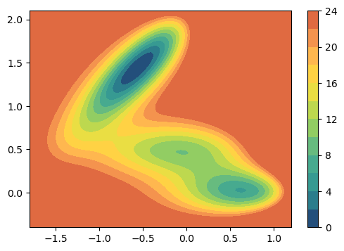
Here we will give a brief overview of the process of training a data-driven collective variable with mlcolvar. As example we will perform a simple regression task for a particle in a 2D toy model potential named Muller-Brown.

# Colab setup
import os

if os.getenv("COLAB_RELEASE_TAG"):
    import subprocess
    subprocess.run('wget https://raw.githubusercontent.com/luigibonati/mlcolvar/main/colab_setup.sh', shell=True)
    cmd = subprocess.run('bash colab_setup.sh TUTORIAL', shell=True, stdout=subprocess.PIPE)
    print(cmd.stdout.decode('utf-8'))

from mlcolvar.utils.plot import muller_brown_potential, plot_isolines_2D

plot_isolines_2D(muller_brown_potential,levels=12,max_value=24)

/Users/luigi/opt/anaconda3/envs/pytorch13/lib/python3.9/site-packages/tqdm/auto.py:21: TqdmWarning: IProgress not found. Please update jupyter and ipywidgets. See https://ipywidgets.readthedocs.io/en/stable/user_install.html
  from .autonotebook import tqdm as notebook_tqdm

<Axes: >

Outline

Typically, the process of constructing a data-driven CV requires the following ingredients:

1. a dataset (with input features and possibly targets or labels)

2. a model (e.g. a neural network) and an objective function.

Once we have them, we can combine them and optimize the CV (via a trainer object).

Finally, we can export the CV in order to be deployed in PLUMED.

Load files

We will load a COLVAR file produced by PLUMED which contains:

• the descriptors (features) which will be used as input of our model, in this case x and y coordinates of the particle

• the quantity to be reproduced (target) which in this case is the potential energy

To do this we can use the load_dataframe function contained in the mlcolvar.utils.io module.

from mlcolvar.utils.io import load_dataframe

filename = "data/muller-brown/unbiased/high-temp/COLVAR"
df = load_dataframe(filename)
df.head()

	time	p.x	p.y	p.z	ene	pot.bias	pot.ene_bias	lwall.bias	lwall.force2	uwall.bias	uwall.force2
0	0.0	0.500000	0.000000	0.0	6.580981	6.580981	6.580981	0.0	0.0	0.0	0.0
1	1.0	0.285803	0.351447	0.0	11.506740	11.506740	11.506740	0.0	0.0	0.0	0.0
2	2.0	-0.004293	0.590710	0.0	11.821637	11.821637	11.821637	0.0	0.0	0.0	0.0
3	3.0	-0.530208	0.714688	0.0	16.812886	16.812886	16.812886	0.0	0.0	0.0	0.0
4	4.0	-1.015236	0.978306	0.0	8.821514	8.821514	8.821514	0.0	0.0	0.0	0.0

Create dataset

We can now create the dataset which will be used to optimize the CV. To do this we can use the DictDataset implemented in the mlcolvar.data module. In case of supervised regression task the keys should be ‘data’ and ‘target’.

from mlcolvar.data import DictDataset
from torch import Tensor

# define input and target features
X = df.filter(regex='p.x|p.y').values     #x,y coordinates
y = df[['ene']].values                    #target energy

# create dataset specifying a dictionary
dataset = DictDataset(dict(data=Tensor(X),target=Tensor(y)))
dataset

DictDataset( "data": [5001, 2], "target": [5001, 1] )

In order to avoid overfitting (i.e. learning to reproduce the training dataset but without the ability to generalize to similar data), it is always good to split the training data into training and validation.

Here we use the lightning framework which takes care of these aspects through an object called DataModule. This takes a dataset and creates training, validation (and optionally also testing) dataloaders which are used by pytorch in the training loop. They are responsible also for dividing the data in batches, shuffling the data and so on, but all of this happens under the hood. We implemented a DictModule which takes as input the dataset which we created above, as well as an indication on how to split data in train and validation sets (here we use 80/20% ratio.)

from mlcolvar.data import DictModule

datamodule = DictModule(dataset,lengths=[0.8,0.2],batch_size=1024)
datamodule

DictModule(dataset -> DictDataset( "data": [5001, 2], "target": [5001, 1] ),
                     train_loader -> DictLoader(length=0.8, batch_size=1024, shuffle=True),
                     valid_loader -> DictLoader(length=0.2, batch_size=1024, shuffle=True))

Define the model

Having organized the data we can now the define the model that we are going to optimize in order to accomplish our regression task. The cvs are implemented in the mlcolvar.cvs module. In particular we are going to use a RegressionCV, which is implemented as a pytorch lightning module. It is composed by two blocks which are executed one after the other: ‘norm_in’ and ‘nn’. The first is a normalization layer which standardize the data based on statistics on the training set, the second the actual FeedForward neural network. These blocks can be customized by passing a dictionary of keyword arguments as described below.

Here we will use a feedforward neural network with three layers and [25,50,25] nodes per layer.

from mlcolvar.cvs import RegressionCV

# specify number of nodes per layer (including input and output dimensions)
layers = [X.shape[1],25,50,25,1]

# specify options for the nn block
nn_args = {'activation': 'relu'}
# specify options for the normalization layer (can be disabled by setting the norm args equal to None or False)
norm_args = {}

model = RegressionCV (layers, options={'norm_in':norm_args , 'nn': nn_args} )
model

RegressionCV(
  (norm_in): Normalization(in_features=2, out_features=2, mode=mean_std)
  (nn): FeedForward(
    (nn): Sequential(
      (0): Linear(in_features=2, out_features=25, bias=True)
      (1): ReLU(inplace=True)
      (2): Linear(in_features=25, out_features=50, bias=True)
      (3): ReLU(inplace=True)
      (4): Linear(in_features=50, out_features=25, bias=True)
      (5): ReLU(inplace=True)
      (6): Linear(in_features=25, out_features=1, bias=True)
    )
  )
)

The loss function is embedded inside the CV object, for a RegressionCV the default is the Mean Square Error (MSE), you will see how to customize it in the following tutorials.

Define the trainer

The last ingredient that we need to define is a lightning Trainer, which ties together the module and the datamodule and performs the training/validation loop. This can be customized with all Lightning features, from logging the metrics to TensorBoard or using EarlyStopping or Learning Rate schedulers. In addition, it can be used to specify the devices to be used for training the CVs, without any extra modification to the code.

In this simple example we will only use a MetricsCallback to save the metrics into a dictionary as well as EarlyStopping criterion acting on the “valid_loss” (it will automatically stop the training after the validation loss does not increase for patience epochs.)

from lightning import Trainer
from lightning.pytorch.callbacks.early_stopping import EarlyStopping
from mlcolvar.utils.trainer import MetricsCallback

# define callbacks
metrics = MetricsCallback()
early_stopping = EarlyStopping(monitor="valid_loss", patience=10, min_delta=1e-5)

# define trainer
trainer = Trainer(callbacks=[metrics, early_stopping],
                     logger=None, enable_checkpointing=False) #disable logger and checkpointing in this tutorial

GPU available: False, used: False
TPU available: False, using: 0 TPU cores
IPU available: False, using: 0 IPUs
HPU available: False, using: 0 HPUs

Optimize it!

Finally we can call the fit method of the trainer and optimize our model!

trainer.fit( model, datamodule )

/Users/luigi/opt/anaconda3/envs/pytorch13/lib/python3.9/site-packages/lightning/loops/utilities.py:70: PossibleUserWarning: `max_epochs` was not set. Setting it to 1000 epochs. To train without an epoch limit, set `max_epochs=-1`.
  rank_zero_warn(

  | Name   | Type          | Params | In sizes | Out sizes
----------------------------------------------------------------
0 | norm_in | Normalization | 0      | [2]      | [2]
1 | nn     | FeedForward   | 2.7 K  | [2]      | [1]
----------------------------------------------------------------
2.7 K     Trainable params
0         Non-trainable params
2.7 K     Total params
0.011     Total estimated model params size (MB)

/Users/luigi/opt/anaconda3/envs/pytorch13/lib/python3.9/site-packages/lightning/loops/fit_loop.py:280: PossibleUserWarning: The number of training batches (4) is smaller than the logging interval Trainer(log_every_n_steps=50). Set a lower value for log_every_n_steps if you want to see logs for the training epoch.
  rank_zero_warn(

Epoch 471: 100%|██████████| 4/4 [00:00<00:00, 46.14it/s, v_num=8]

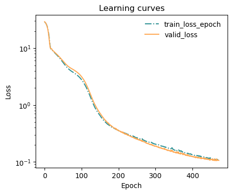
The train/valid losses are saved into the metrics object. We can use an helper function to plot them:

from mlcolvar.utils.plot import plot_metrics

ax = plot_metrics(metrics.metrics,
                  keys=['train_loss_epoch','valid_loss'],
                  linestyles=['-.','-'], colors=['fessa1','fessa5'],
                  yscale='log')

Analyze the results

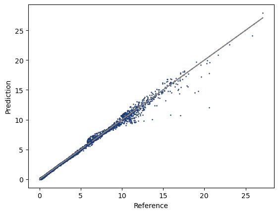
Once the model is optimized, we can directly use it to predict the cv for new data. And of course, we can compare the predicted vs reference data.

from torch import no_grad # allows for inference without gradients

# predict data
model.eval()
with no_grad():
    y_pred = model(Tensor(X))

# compare with reference
import matplotlib.pyplot as plt
_,ax = plt.subplots(dpi=100)
ax.scatter(y,y_pred,s=1,color='fessa0',alpha=0.8)
ax.plot(y,y,linestyle='--',color='grey')
#ax.set_xlim(-0.1,1.1)
#ax.set_ylim(-0.1,1.1)
ax.set_xlabel('Reference')
ax.set_ylabel('Prediction')

Text(0, 0.5, 'Prediction')

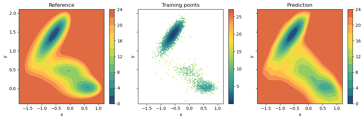
Since this is a two-dimensional model potential we can also compare the results in the (x,y) space. To do that we need to compute the isolines of the CV and compare with the true potential. The prediction is actually rather accurate, except for the regions where few if any data points are available.

fig,axs = plt.subplots(1,3,dpi=100,figsize=(12,4),sharex=True,sharey=True)
for ax,title in zip(axs,['Reference','Training points','Prediction']):
    ax.set_title(title)
    ax.set_xlabel('x')
    ax.set_ylabel('y')

plot_isolines_2D(muller_brown_potential,levels=12,max_value=24,ax=axs[0])
pp = axs[1].scatter(X[:,0],X[:,1],c=y[:,0],s=1,alpha=1,cmap='fessa')
plt.colorbar(pp,ax=axs[1])
plot_isolines_2D(model,levels=12,max_value=24,ax=axs[2])
plt.tight_layout()

Deploy the model in PLUMED

In order to deploy the model to PLUMED we first need to compile it TorchScript (see torch.jit). We will trace the model, meaning that all of the instructions that are executed in an example workflow will be compiled in a python-independent format. Once again we can use lightning wrapper to do so, and just call the method to_torchscript.

model.to_torchscript('model.ptc',method="trace")

Then an example input file to evaluate and print the CV from PLUMED could be:

# ------------- plumed.dat -------------
p:  POSITION ATOM=1
cv: PYTORCH_MODEL FILE=model.ptc ARG=p.x,p.y

PRINT STRIDE=100 ARG=cv.*
# --------------------------------------

For complete details on how you should use your data-driven CVs in PLUMED you should check the PLUMED documentation!

You made it to the end! This first tutorial was designed to give an overview on the process of training data-driven CVs with mlcolvar. You can now navigate through the CV-specific tutorials which describe the different approaches which are implemented as well as information on how to customize the CVs and the training.