DeepTICA: Alanine dipeptide from multithermal simulation

Reference paper: Bonati, Piccini and Parrinello, PNAS (2020) [arXiv].

Prerequisite: DeepTICA tutorial.

Setup

# Colab setup
import os

if os.getenv("COLAB_RELEASE_TAG"):
    import subprocess
    subprocess.run('wget https://raw.githubusercontent.com/luigibonati/mlcolvar/main/colab_setup.sh', shell=True)
    cmd = subprocess.run('bash colab_setup.sh EXAMPLE', shell=True, stdout=subprocess.PIPE)
    print('Done!')

# IMPORT PACKAGES
import torch
import lightning
import numpy as np
import matplotlib.pyplot as plt

# Set seed for reproducibility
torch.manual_seed(42)

<torch._C.Generator at 0x7fe41d2d90f0>

Alanine dipeptide: OPES Multithermal -> DeepTICA

In this example we illustrate a case of applying DeepTDA to a biased simulation, taken from the DeepTICA manuscript. In particular, we will use the alanine dipeptide example in which we collect the simulations from the OPES multithermal simulation (which thus do not require to define a trial CV).

Load data

First we load the COLVAR file(s) containing the weights of the OPES simulation and the input features, in this case they are the 45 interatomic distances between heavy atoms.

We discard the initial part of the simulation to put ourselves in the quasi-static regime, which is very quickly reached by OPES (it can be monitored by looking at the DELTAFS file for the multicanonical simulation).

The data is downloaded from the Github repository associated with the manuscript.

import pandas as pd
from mlcolvar.utils.io import load_dataframe
from mlcolvar.utils.timelagged import create_timelagged_dataset
from mlcolvar.data import DictModule

# load colvar files containing weights of the OPES simulations as well as the driver with the input features
opes = load_dataframe('https://raw.githubusercontent.com/luigibonati/deep-learning-slow-modes/main/data/ala2-multi/1_opes_multi/COLVAR',
                      start=15000,stop=50000)
feat = load_dataframe('https://raw.githubusercontent.com/luigibonati/deep-learning-slow-modes/main/data/ala2-multi/2_training_cvs/COLVAR_DRIVER',
                          start=15000,stop=50000)

# concatenate them
df = pd.concat([opes, feat[[i for i in feat.columns if (i not in opes.columns)]]], axis=1)

df

	time	phi	psi	ene	opes.bias	walker	d1	d2	d3	d4	...	d36	d37	d38	d39	d40	d41	d42	d43	d44	d45
0	15000.0	-1.24937	0.540396	-53.9859	1.725970	0	0.1522	0.233868	0.244634	0.382245	...	0.258908	0.277790	0.379264	0.498986	0.1229	0.1335	0.246437	0.225420	0.283532	0.1449
1	15001.0	-1.50515	1.438650	43.3469	-30.144900	0	0.1522	0.235165	0.241863	0.375188	...	0.255153	0.295903	0.367831	0.502540	0.1229	0.1335	0.252509	0.223947	0.291499	0.1449
2	15002.0	-1.29419	1.730900	-18.3581	-0.562392	0	0.1522	0.244679	0.231301	0.370506	...	0.252451	0.285218	0.363133	0.486784	0.1229	0.1335	0.241549	0.226609	0.276819	0.1449
3	15003.0	-2.53166	2.657820	-23.8477	0.715870	0	0.1522	0.234523	0.246725	0.382103	...	0.250699	0.317424	0.312897	0.441096	0.1229	0.1335	0.246988	0.230302	0.292824	0.1449
4	15004.0	-2.15710	2.395360	11.5125	-14.231600	0	0.1522	0.234793	0.251158	0.383453	...	0.262807	0.326766	0.339187	0.479339	0.1229	0.1335	0.251390	0.224343	0.292820	0.1449
...	...	...	...	...	...	...	...	...	...	...	...	...	...	...	...	...	...	...	...	...	...
34995	49995.0	-1.19288	0.532025	-28.4388	1.276180	0	0.1522	0.232503	0.245793	0.382845	...	0.258933	0.285152	0.382687	0.493388	0.1229	0.1335	0.242527	0.216974	0.264171	0.1449
34996	49996.0	-1.31044	-0.023952	-33.1943	1.544550	0	0.1522	0.237438	0.245095	0.377144	...	0.246469	0.276428	0.354929	0.473255	0.1229	0.1335	0.249179	0.221805	0.281781	0.1449
34997	49997.0	-1.66419	2.736990	-32.5060	1.518380	0	0.1522	0.240949	0.244720	0.385074	...	0.253170	0.327638	0.315540	0.453209	0.1229	0.1335	0.240503	0.223382	0.272337	0.1449
34998	49998.0	-1.71317	2.573260	19.0074	-17.968700	0	0.1522	0.240229	0.247424	0.383137	...	0.245395	0.310855	0.318514	0.438564	0.1229	0.1335	0.243461	0.226024	0.279091	0.1449
34999	49999.0	-1.26937	2.127590	7.2590	-12.103300	0	0.1522	0.241292	0.235914	0.373783	...	0.254010	0.289084	0.355414	0.456283	0.1229	0.1335	0.247204	0.220562	0.278850	0.1449

35000 rows × 51 columns

# Select input features
X = df.filter(regex='d').values
n_input = X.shape[1]

print(X.shape)

(35000, 45)

Create time-lagged dataset

Compute weights for time rescaling

Here we extract the time \(t\), the energy \(E\) (needed for the multicanonical reweight [1]) and the bias \(V\) from the COLVAR file. We then calculate the weights as:

NB: note that if simulation temperature \(\beta_0\) is equal to the reweighting one \(\beta\) the multicanonical reweight coincides with the standard umbrella sampling-like case.

Once we have computed the weights, we rescale the time at step \(k\) by using the instantaneus acceleration:

\[dt'_k = w_k\ dt\]

and then compute the cumulative rescaled time:

\[t'_k = \sum_{i=0} ^k dt'_i\]

[1] Invernizzi, Piaggi, and Parrinello. “Unified approach to enhanced sampling.” Physical Review X 10.4 (2020): 041034.

---

Parameter	Type	Description
multicanonical	bool	flag to determine if using a standard reweight (false) or a multicanonical one (true)
temp	float	reweighting temperature
temp0	float	simulation temperature (only needed if multicanonical == True)

#------------- PARAMETERS -------------
multicanonical    = True
temp              = 300.
temp0             = 300.
#--------------------------------------

# Calculate inverse temperature
kb=0.008314
beta=1./(kb*temp)
beta0=1./(kb*temp0)

# Extract cvs from df

t = df['time'].values # save time
ene = df['ene'].values.astype(np.float64) # store energy as long double
bias = df.filter(regex='.bias').values.sum(axis=1) # Load *.bias columns and sum them

# Compute log-weights for time reweighting
logweights = beta*bias

if multicanonical:
    ene -= np.mean(ene) #first shift energy by its mean value
    logweights += (beta0-beta)*ene

In order to train the Deep-TICA CVs we will need to compute the time-lagged covariance matrices in the rescaled time \(t'\). The standard way is to look for configurations which are distant a lag-time \(\tau\) in the time series. However, in the rescaled time the time-series is exponentially unevenly spaced. Hence, a naive search will lead to severe numerical issue. To address this, we use the algorithm proposed in [2]. In a nutshell, this method assume that the observable \(O(t'_k)\) have the same value from scaled time \(t'_k\) to \(t'_{k+1}\). This leads to weighting each pair of configurations based both on the rescaled time around \(t'_k\) and \(t'_k+\tau\) (see supp. information of [2] for details). All of this is done under the hood in the function find_time_lagged_configurations. To generate the training set we use the function create_time_lagged_dataset which searches for the pairs of configurations and the corresponding weight.

[2] Yang and Parrinello. “Refining collective coordinates and improving free energy representation in variational enhanced sampling.” Journal of chemical theory and computation 14.6 (2018): 2889-2894.

---

Parameter	Type	Description
lag_time	float	lag_time for the calculation of the covariance matrices [in rescaled time]
n_train	int	number of training configurations
n_valid	int	number of validation configurations

#------------- PARAMETERS -------------
lag_time = 1.
#--------------------------------------

# create dataset
dataset = create_timelagged_dataset(X,t,lag_time=lag_time,logweights=logweights,progress_bar=True)

# create datamodule (split train valid)
datamodule = DictModule(dataset,lengths=[0.8,0.2],random_split=False,shuffle=False)

datamodule

100%|██████████| 34997/34997 [00:03<00:00, 11180.12it/s]
/home/lbonati@iit.local/work/code/mlcolvar120/mlcolvar/utils/timelagged.py:186: UserWarning: Creating a tensor from a list of numpy.ndarrays is extremely slow. Please consider converting the list to a single numpy.ndarray with numpy.array() before converting to a tensor. (Triggered internally at ../torch/csrc/utils/tensor_new.cpp:275.)
  x_t = torch.stack(x_t) if type(x) == torch.Tensor else torch.Tensor(x_t)
/home/lbonati@iit.local/work/code/mlcolvar120/mlcolvar/data/datamodule.py:133: UserWarning: A torch.generator was provided but it is not used with random_split=False
  warnings.warn(

DictModule(dataset -> DictDataset( "data": [66163, 45], "data_lag": [66163, 45], "weights": [66163], "weights_lag": [66163] ),
                     train_loader -> DictLoader(length=0.8, batch_size=0, shuffle=False),
                     valid_loader -> DictLoader(length=0.2, batch_size=0, shuffle=False))

Define model

from mlcolvar.cvs import DeepTICA

n_components = 2
nn_layers = [n_input, 30, 30, n_components]
options= {'nn': {'activation': 'tanh'}}

model = DeepTICA(nn_layers, options=options)
model

DeepTICA(
  (loss_fn): ReduceEigenvaluesLoss()
  (norm_in): Normalization(in_features=45, out_features=45, mode=mean_std)
  (nn): FeedForward(
    (nn): Sequential(
      (0): Linear(in_features=45, out_features=30, bias=True)
      (1): Tanh()
      (2): Linear(in_features=30, out_features=30, bias=True)
      (3): Tanh()
      (4): Linear(in_features=30, out_features=2, bias=True)
    )
  )
  (tica): TICA(in_features=2, out_features=2)
)

Define Trainer & Fit

from lightning.pytorch.callbacks.early_stopping import EarlyStopping
from mlcolvar.utils.trainer import MetricsCallback

# define callbacks
metrics = MetricsCallback()
early_stopping = EarlyStopping(monitor="valid_loss", min_delta=1e-3, patience=10)

# define trainer
trainer = lightning.Trainer(callbacks=[metrics, early_stopping],
                     max_epochs=None, logger=None, enable_checkpointing=False)

# fit
trainer.fit( model, datamodule )

GPU available: True (cuda), used: True
TPU available: False, using: 0 TPU cores
IPU available: False, using: 0 IPUs
HPU available: False, using: 0 HPUs
/home/lbonati@iit.local/software/mambaforge/envs/mlcolvar111/lib/python3.10/site-packages/lightning/pytorch/trainer/connectors/logger_connector/logger_connector.py:75: Starting from v1.9.0, `tensorboardX` has been removed as a dependency of the `lightning.pytorch` package, due to potential conflicts with other packages in the ML ecosystem. For this reason, `logger=True` will use `CSVLogger` as the default logger, unless the `tensorboard` or `tensorboardX` packages are found. Please `pip install lightning[extra]` or one of them to enable TensorBoard support by default
/home/lbonati@iit.local/software/mambaforge/envs/mlcolvar111/lib/python3.10/site-packages/lightning/pytorch/loops/utilities.py:73: `max_epochs` was not set. Setting it to 1000 epochs. To train without an epoch limit, set `max_epochs=-1`.
You are using a CUDA device ('NVIDIA GeForce RTX 3090') that has Tensor Cores. To properly utilize them, you should set `torch.set_float32_matmul_precision('medium' | 'high')` which will trade-off precision for performance. For more details, read https://pytorch.org/docs/stable/generated/torch.set_float32_matmul_precision.html#torch.set_float32_matmul_precision
LOCAL_RANK: 0 - CUDA_VISIBLE_DEVICES: [0]

  | Name    | Type                  | Params | In sizes | Out sizes
-------------------------------------------------------------------------
0 | loss_fn | ReduceEigenvaluesLoss | 0      | ?        | ?
1 | norm_in | Normalization         | 0      | [1, 45]  | [1, 45]
2 | nn      | FeedForward           | 2.4 K  | [1, 45]  | [1, 2]
3 | tica    | TICA                  | 0      | [1, 2]   | [1, 2]
-------------------------------------------------------------------------
2.4 K     Trainable params
0         Non-trainable params
2.4 K     Total params
0.009     Total estimated model params size (MB)

[Warning] Normalization: the following features have a range of values < 1e-6: tensor([[ 0],
        [ 9],
        [10],
        [24],
        [30],
        [31],
        [39],
        [40],
        [44]])

/home/lbonati@iit.local/software/mambaforge/envs/mlcolvar111/lib/python3.10/site-packages/lightning/pytorch/loops/fit_loop.py:298: The number of training batches (1) is smaller than the logging interval Trainer(log_every_n_steps=50). Set a lower value for log_every_n_steps if you want to see logs for the training epoch.

Epoch 398: 100%|██████████| 1/1 [00:00<00:00, 30.05it/s, v_num=5]

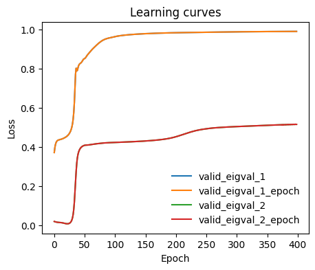
We can monitor how the individual eigenvalues are optimized during training.

from mlcolvar.utils.plot import plot_metrics

ax = plot_metrics(metrics.metrics,
                  keys=[x for x in  metrics.metrics.keys() if 'valid_eigval' in x],#['train_loss_epoch','valid_loss'],
                  #linestyles=['-.','-'], colors=['fessa1','fessa5'],
                  yscale='linear')

Normalize output

For convenience, we standardize the CVs to be between -1 and 1.

from mlcolvar.core.transform import Normalization
from mlcolvar.core.transform.utils import Statistics

#X = dataset[:]['data']
with torch.no_grad():
    model.postprocessing = None # reset
    s = model(torch.Tensor(X))

norm =  Normalization(n_components, mode='min_max', stats = Statistics(s) )
model.postprocessing = norm

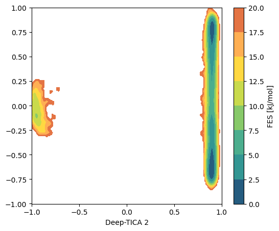
Compute FES

We can plot the free energy profile along the selected CVs. First we compute it in the 2D space, from which we learn that the first TICA refers to the transition between two long-lived metastable states, while the second the faster transitions within the left basin.

from mlcolvar.utils.fes import compute_fes

fig,ax = plt.subplots(1,1,figsize=(6,5),dpi=100)

# compute cvs
with torch.no_grad():
    s = model(torch.Tensor(X)).numpy()

w = np.exp(logweights)
fes,grid,bounds,error = compute_fes(s,
                                    weights=w,
                                    temp=300,
                                    blocks=1,
                                    bandwidth=0.01, scale_by='range',
                                    plot=True, plot_max_fes=20, ax = ax, eps=1e-10)

ax.set_xlabel('Deep-TICA 1')
ax.set_xlabel('Deep-TICA 2')

Text(0.5, 0, 'Deep-TICA 2')

We can also plot the free energy profiles along each component. From the 2D FES above we understand that for the second CV we need to compute the FES only for the points in which the first CV is < 0, in order to describe the barrier between the faster states.

from mlcolvar.utils.fes import compute_fes

fig,axs = plt.subplots(1,n_components,figsize=(6*n_components,5),dpi=100)

for i in range(n_components):
    w = np.exp(logweights)

    # restrict the second CV to the points in which the first is < 0
    mask = np.ones(len(s), dtype=bool) if i==0 else s[:, 0] < 0

    fes,grid,bounds,error = compute_fes(s[mask,i],
                                        weights=w[mask],
                                        temp=300,
                                        blocks=2,
                                        bandwidth=0.02,
                                        scale_by='range',
                                        plot=True,
                                        plot_max_fes=50,
                                        backend='sklearn', # the default=KDEpy is faster but may be unstable for latest python/numpy builds
                                        ax = axs[i])
    axs[i].set_xlabel('Deep-TICA '+str(i+1))

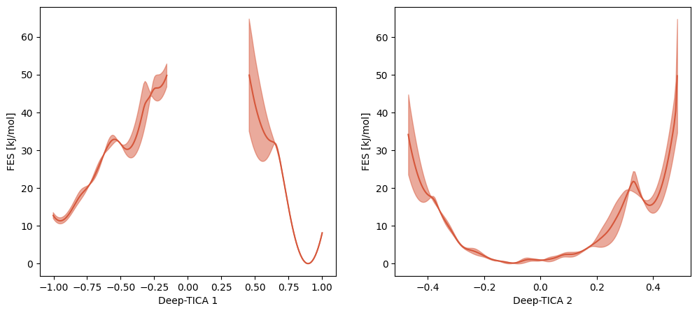
Note that the huge uncertainty on the free energy barrier is due to the lack of points between the states in the multithermal simulation.

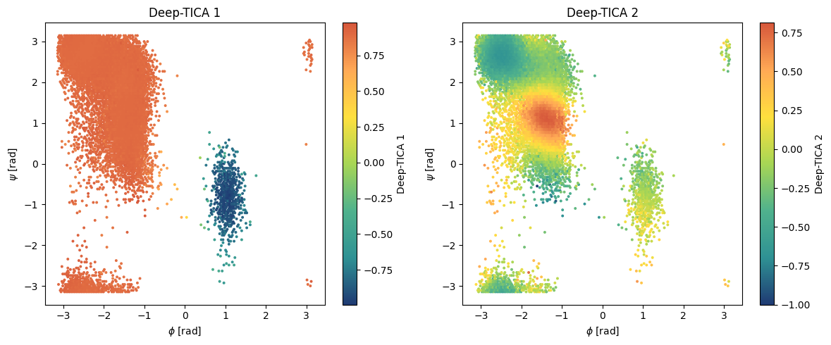
Plot CVs isolines in \(\phi-\psi\) space

To understand to what states the CVs refer to, we can visualize them in the Ramachandran plot (\(\phi\) and \(\psi\)).

# Hexbin plot in physical space
fig,axs = plt.subplots(1,n_components,figsize=(6*n_components,5),dpi=100)

x = df['phi'].values
y = df['psi'].values

# compute cvs
with torch.no_grad():
    s = model(torch.Tensor(X)).numpy()

for i,ax in enumerate(axs):
    pp = ax.hexbin(x,y,C=s[:,i],gridsize=150,cmap='fessa')
    cbar = plt.colorbar(pp,ax=ax)
    ax.set_title('Deep-TICA '+str(i+1))
    ax.set_xlabel(r'$\phi$ [rad]')
    ax.set_ylabel(r'$\psi$ [rad]')
    cbar.set_label('Deep-TICA '+str(i+1))

plt.tight_layout()
plt.show()

You can try out also the other examples reported in the paper, such as applying DeepTICA to a simulation biasing a bad CV (the \(\psi\) dihedral angle).